Week 3.5 - Deriving 4th order approximation of a 2nd order derivative using Taylor Table method

Objective:

a)To write a code to calculate error values for central differencing , right skew and left skew method of approximations of fourth order derivatives

of given function .

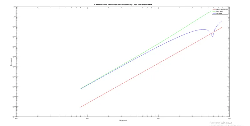
b) To plot dx Vs error graphs for all 3 cases.

Theory :

According to Taylor series , we can calculate 4th order approximations by using below equations

a) for central differencing method ,

n=p+q-1 =4+2-1 = 5

`d^2/dx^2 f(x)` = a f(i-2) +b f(i-1)+c f(i)+d f(i+1)+e f(i+2) -------------------------------equation(1)

	f(i)	`triangle x`f'(x)	`triangle x^2 f''(x)`	`trianglex^3 f'''(x)`	`triangle x^4 f''''(x)`
a f(i-2)	a	-2a	4a/2	-8a/6	16a/24
b f(i-2)	b	-b	b/2	-b/6	b/24
c f(i)	c	0	0	0	0
d f(i+1)	d	d	d/2	d/6	d/24
e f(i+2)	e	2e	4e/2	8e/6	16e/24
	0	0	1	0	0

`del^2/(delx)^2f(x)` = f(x) + `triangle x f'(x)`+`triangle x^2 f''(x)`/2! +`triangle x^3 f'''(x)`/3! +`triangle x^4 f''''(x)`/4!

We can obtain equations for a,b,c,d,e from this table

a+b+c+d+e=0

-2a-b+0+d+2e = 0

4a/2 +b/2+0+d/2+4e/2=1

-8/6a-b/6+0+d/6+8e/6=0

16/24a+b/24+0+d/24+16e/24=0

A=[ 1 1 1 1 1 ;
-2 -1 0 1 2;
2 1/2 0 1/2 2;
-4/3 -1/6 0 1/6 4/3;
2/3 1/24 0 1/24 2/3]

B=[0;0;1;0;0]

X= [A] inverse *[B]

hence we can calculate approximation by substituting these values on 1st equation .

b) For right skew method,

n=p+q =4+2=6

`del^2/(delx)^2 f(x)` = a f(i)+b f(i+1) +c f(i+2) +d f(i+3) +e f(i+4) + g f(i+5)-------------------------equation(2`

	f(x)	`triangle x f'(x)`	`triangle x^2 f''(x)`	`triangle x^3 f'''(x)`	`triangle x^4 f''''(x)`	`trianglex^5 f'''''(x)`
a(i)	a	0	0	0	0	0
b(i+1)	b	b	b/2	b/6	b/24	b/120
c(i+2)	c	2c	4c/2	8c/6	16c/24	32c/120
d(i+3)	d	3d	9d/2	27d/6	81d/24	243d/120
e(i+4)	e	4e	16e/2	64e/6	256e/24	1024e/120
g(i+5)	g	5g	25g/2	125g/6	625g/24	3125g/120
	0	0	1	0	0	0

`del^2/(delx)^2f(x)` = f(x) + `triangle x f'(x)`+`triangle x^2 f''(x)`/2! +`triangle x^3 f'''(x)`/3! +`triangle x^4 f''''(x)`/4! +`triangle x^5 f'''''(x)`/5!

a+b+c+d+e+g=0

0+b+2c+3d+4e+5g=0

0+b/2+4/2c+9/2e+16/2e+25g/2 =1

0+b/6+8c/6+27d/6+64e/6+125g/6=0

0+b/24+16c/24+81d/24+256e/24+625g/24=0

0+b/120+32c/120+243d/120+1024e/120+3125g/120=0

A= [ 1 1 1 1 1 1;
0 1 2 3 4 5;
0 1/2 2 9/2 8 25/2;
0 1/6 4/3 27/6 64/6 125/6;
0 1/24 2/3 81/24 256/24 625/24;
0 1/120 16/60 243/120 1024/120 3125/120; ]
B= [0;0;1;0;0;0]

X=[A] inverse*[B]

Hence we can compute the approximation by substituting these values on equation(2)

C) For left skew method

n=p+q =4+2=6

del^2/(delx)^2 f(x)` = a f(i)+b f(i-1) +c f(i-2) +d f(i-3) +e f(i-4) + g f(i-5)-----------------equation(3)

	f(x)	`triangle x f'(x)`	`triangle x^2 f''(x)`	`triangle x^3 f'''(x)`	`triangle x^4 f''''(x)`	`trianglex^5 f'''''(x)`
a(i)	a	0	0	0	0	0
b(i+1)	b	-b	b/2	-b/6	b/24	-b/120
c(i+2)	c	-2c	4c/2	-8c/6	16c/24	-32c/120
d(i+3)	d	-3d	9d/2	-27d/6	81d/24	-243d/120
e(i+4)	e	-4e	16e/2	-64e/6	256e/24	-1024e/120
g(i+5)	g	-5g	25g/2	-125g/6	625g/24	-3125g/120
	0	0	1	0	0	0

`del^2/(delx)^2f(x)` = f(x) + `triangle x f'(x)`+`triangle x^2 f''(x)`/2! +`triangle x^3 f'''(x)`/3! +`triangle x^4 f''''(x)`/4! +`triangle x^5 f'''''(x)`/5!

a+b+c+d+e+g=0

0-b-2c-3d-4e-5g=0

0+b/2+4/2c+9/2e+16/2e+25g/2 =1

0-b/6-8c/6-27d/6-64e/6-125g/6=0

0+b/24+16c/24+81d/24+256e/24+625g/24=0

0-b/120-32c/120-243d/120-1024e/120-3125g/120=0

A= [ 1 1 1 1 1 1;
0 -1 - 2 -3 -4 -5;
0 1/2 2 9/2 8 25/2;
0 -1/6 -4/3 -27/6 -64/6 - 125/6;
0 1/24 2/3 81/24 256/24 625/24;
0 -1/120 -16/60 -243/120 -1024/120 -3125/120; ]
B= [0;0;1;0;0;0]

X=[A] inverse*[B]

By substituting these values in equation (3), we can compute the approximations

Program Logic :

%f(x)=exp(x)*cos(x) : Function f(x)
%f'(x)=exp(x)*-sin(x) + cos(x)exp(x) : `del/(delx) f(x)`
%f''x= exp(x)*-cos(x)-sin(x)*exp(x)+cos(x)*exp(x)+exp(x)*-sin(x) : `del^2/(delx^2) f(x)`
x=pi/3; : Assigning value of x
dx=linspace(pi/4,pi/400,20); : To create an array for dx with 20 values varying from pi/4 to pi/400
ad = -2*sin(x)*exp(x); : Equation to calculate analytical derivative

for i=1:length(dx) : for loop to calcuate errors for varying values of dx
%calling functions to return respective error values
FOCD(i)= focd(x,dx(i)); : Calling function focd with x and dx(i) as inputs
RSKEW(i)=rskew(x,dx(i)); :Calling function rskew with x and dx(i) as inputs
LSKEW(i)=lskew(x,dx(i)); :Calling function lskew with x and dx(i) as inputs
end : End of for loop

%to plot
figure(1)
loglog(dx,FOCD,'r'); : To plot log graph of dx Vs error of central deifferencing
hold on : To hold on to plot
loglog(dx,RSKEW,'g'); : To plot log graph of dx vs error of right skew
loglog(dx,LSKEW,'b'); : To plot log graph of dx vs error of left skew
title('dx Vs Error values for 4th order central differencing , right skew and left skew') : To name the plot
xlabel ('Value of dx') : To name x axis
ylabel('Error value ') : To name y axis
legend('Central differencing','Right skew','Left skew'); : To mark legends

function retval1 = focd (x,dx) : Function definition of focd
ad = -2*sin(x)*exp(x); : equation for analytical derivative

A=[ 1 1 1 1 1; : Matrix [A] from taylors table
-2 -1 0 1 2;
2 1/2 0 1/2 2;
-4/3 -1/6 0 1/6 4/3;
2/3 1/24 0 1/24 2/3]
B= [0;0;1;0;0]; : Solution Matirx [B]
%X=inv(A)*B;
X=linsolve(A,B); : Matrix with values of co-efficients a,b,c,d,e
term1=X(1)*(exp(x-(2*dx))*cos(x-(2*dx))); : Part 1 of solution equation RHS
term2=X(2)*(exp(x-dx)*cos(x-dx)); :Part 2 of solution equation RHS
term3=X(3)*(exp(x)*cos(x)); :Part 3 of solution equation RHS
term4=X(4)*(exp(x+dx)*cos(x+dx)); :Part 4 of solution equation RHS
term5=X(5)*(exp(x+(2*dx))*cos(x+(2*dx))); :Part 5 of solution equation RHS
y=(term1+term2+term3+term4+term5)/(dx^2); :Final solution equation
retval1=abs(y-ad); :equation to calculate absolute value of error
endfunction :end of function

function retval2 = rskew (x,dx) : definition of function rskew with input x and dx
ad = -2*sin(x)*exp(x); : equation for analytical derivative

A=[1 1 1 1 1 1; :Matrix [A] from taylors table
0 1 2 3 4 5;
0 1/2 2 9/2 8 25/2;
0 1/6 4/3 27/6 64/6 125/6;
0 1/24 2/3 81/24 256/24 625/24;
0 1/120 16/60 243/120 1024/120 3125/120; ]
B= [0;0;1;0;0;0] : Solution Matirx [B]
% X=rats(linsolve(A,B))
X=inv(A)*B; :Matrix with values of co-efficients a,b,c,d,e

term1=X(1)*exp(x)*cos(x); :Part 1 of solution equation RHS
term2=X(2)*exp(x+dx)*cos(x+dx); :Part 2 of solution equation RHS
term3=X(3)*exp(x+2*dx)*cos(x+2*dx); :Part 3 of solution equation RHS
term4=X(4)*exp(x+3*dx)*cos(x+3*dx); :Part 4 of solution equation RHS
term5=X(5)*exp(x+4*dx)*cos(x+4*dx); :Part 5 of solution equation RHS
term6=X(6)*exp(x+5*dx)*cos(x+5*dx); :Part 6 of solution equation RHS
y=(term1+term2+term3+term4+term5+term6)/(dx^2); :Final solution equation
retval2=abs(y-ad); :equation to calculate absolute value of error

endfunction :end of function

The function for lskew is same as that of rskew only difference being in the

a) Matrix A

A=[1 1 1 1 1 1;
0 -1 -2 -3 -4 -5;
0 1/2 2 9/2 16/2 25/2;
0 -1/6 -8/6 -27/6 -64/6 -125/6;
0 1/24 16/24 81/24 256/24 625/24 ;
0 -1/120 -32/120 -243/120 -1024/120 -3125/120 ]

b) Final equation :

term1=X(1)*exp(x)*cos(x);
term2=X(2)*exp(x-dx)*cos(x-dx);
term3=X(3)*exp(x-2*dx)*cos(x-2*dx);
term4=X(4)*exp(x-3*dx)*cos(x-3*dx);
term5=X(5)*exp(x-4*dx)*cos(x-4*dx);
term6=X(6)*exp(x-5*dx)*cos(x-5*dx);
y=(term1+term2+term3+term4+term5+term6)/(dx^2);
retval3=abs(y-ad);

Program Code :

clear all
close all
clc

%f(x)=exp(x)*cos(x)
%f'(x)=exp(x)*-sin(x) + cos(x)exp(x) 
%f''x= exp(x)*-cos(x)-sin(x)*exp(x)+cos(x)*exp(x)+exp(x)*-sin(x)
x=pi/3;
dx=linspace(pi/4,pi/400,20);
ad = -2*sin(x)*exp(x);

%dx=linspace(pi/40,pi/400,20);

for i=1:length(dx)
  %calling functions to return respective error values
FOCD(i)= focd(x,dx(i));
RSKEW(i)=rskew(x,dx(i));
LSKEW(i)=lskew(x,dx(i));
end

%to plot
figure(1)
loglog(dx,FOCD,'r');
hold on
loglog(dx,RSKEW,'g');
loglog(dx,LSKEW,'b');
title('dx Vs Error values for 4th order central differencing , right skew and left skew')
xlabel ('Value of dx')
ylabel('Error value ')
legend('Central differencing','Right skew','Left skew');

Function 1 to calculate using Central differencing

function retval1 = focd (x,dx)
ad = -2*sin(x)*exp(x);

A=[ 1  1  1  1  1;
   -2 -1  0  1  2;
    2 1/2 0  1/2  2;
  -4/3 -1/6 0 1/6 4/3;
   2/3 1/24 0 1/24 2/3]
 B= [0;0;1;0;0];
 %X=inv(A)*B;
 X=linsolve(A,B);
 term1=X(1)*(exp(x-(2*dx))*cos(x-(2*dx)));
 term2=X(2)*(exp(x-dx)*cos(x-dx));
 term3=X(3)*(exp(x)*cos(x));
 term4=X(4)*(exp(x+dx)*cos(x+dx));
 term5=X(5)*(exp(x+(2*dx))*cos(x+(2*dx)));
 y=(term1+term2+term3+term4+term5)/(dx^2);
 retval1=abs(y-ad);
 endfunction

Function 2 to calculate using Right skew

function retval2 = rskew (x,dx)
  ad = -2*sin(x)*exp(x);

A=[1   1   1   1    1   1;
   0   1   2   3    4   5;
   0   1/2  2  9/2  8  25/2;
   0  1/6   4/3  27/6 64/6  125/6;
   0   1/24  2/3  81/24  256/24  625/24;
   0   1/120  16/60  243/120  1024/120  3125/120; ]
 B= [0;0;1;0;0;0]
% X=rats(linsolve(A,B))
 X=inv(A)*B;
 
 term1=X(1)*exp(x)*cos(x);
 term2=X(2)*exp(x+dx)*cos(x+dx);
 term3=X(3)*exp(x+2*dx)*cos(x+2*dx);
 term4=X(4)*exp(x+3*dx)*cos(x+3*dx);
 term5=X(5)*exp(x+4*dx)*cos(x+4*dx);
 term6=X(6)*exp(x+5*dx)*cos(x+5*dx);
 y=(term1+term2+term3+term4+term5+term6)/(dx^2);
 retval2=abs(y-ad);
 
endfunction

3)Function 3 to calculate using left skew

function retval3 = lskew (x,dx)
  ad = -2*sin(x)*exp(x);
A=[1    1    1    1   1     1;
   0    -1   -2   -3   -4   -5;
   0    1/2   2    9/2   16/2   25/2;
   0    -1/6   -8/6   -27/6  -64/6   -125/6;
   0     1/24    16/24    81/24    256/24     625/24  ;
    0     -1/120   -32/120   -243/120    -1024/120    -3125/120   ]
    B=[0 ; 0; 1;0;0;0  ]
    X=inv(A)*B;
    term1=X(1)*exp(x)*cos(x);
 term2=X(2)*exp(x-dx)*cos(x-dx);
 term3=X(3)*exp(x-2*dx)*cos(x-2*dx);
 term4=X(4)*exp(x-3*dx)*cos(x-3*dx);
 term5=X(5)*exp(x-4*dx)*cos(x-4*dx);
 term6=X(6)*exp(x-5*dx)*cos(x-5*dx);
 y=(term1+term2+term3+term4+term5+term6)/(dx^2);
 retval3=abs(y-ad);

endfunction

Results :

1)The error values for 4th order approximation of 2nd order were calculated using all 3 methods for the given function

2) The log graphs were plotted for the same