Week 3.5 - Deriving 4th order approximation of a 2nd order derivative using Taylor Table method

We have to derive the 4th order approximations of the second-order derivative for the following:

1. Skewed right-sided difference
2. Skewed left-sided difference
3. Central difference

Given analytical function exp(x)*cos(x)

Node Calculation:
We need to first have several nodes for each of the differentials to calculate further and make the Taylor table.

N = number of nodes; P = order of derivative; Q = order of approximation

Nodes for left and right side difference = 2 (2nd order derivative) + 4 (4th order approximation)
= 6
Thus, as we can see, the hypothesis equation contains 6 points/nodes for order approximation calculation.

Nodes for central difference = 2 (2nd order derivative) + 4 (4th order approximation) -1
= 5
Similarly, we can see, the hypothesis equation contains 5 points/nodes for order approximation calculation.

Derivation:

• Skewed right-sided difference:

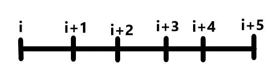
We have first calculated the number of nodes required to solve this differential. Based on that, we've formulated the below equation.
Hypothesis equation = `Deltax^2(d^2u)/dx^2 = a f(i)+bf(i+1)+ cf(i+2) + df(i+3)+ef(i+4)+gf(i+5)`

Taylor Expansion of the terms in the equation:

`a*f(i)=a*f(i)`

`b*f(i+1)=b(f(i)+Deltaxf(i)+(Deltax^2)/(2!)f(i)+(Deltax^3)/(3!)f(i)+(Deltax^4)/(4!)f(i)+ (Deltax^5)/(5!)f(i))`

`c*f(i+2)=c(f(i)+2Deltaxf(i)+(2Deltax)^2/(2!)f(i)+(2Deltax)^3/(3!)f(i)+(2Deltax)^4/(4!)f(i)+ (2Deltax)^5/(5!)f(i))`

`d*f(i+3)=d(f(i)+3Deltaxf(i)+(3Deltax)^2/(2!)f(i)+(3Deltax)^3/(3!)f(i)+(3Deltax)^4/(4!)f(i)+ (3Deltax)^5/(5!)f(i))`

`e*f(i+4)=e(f(i)+4Deltaxf(i)+(4Deltax)^2/(2!)f(i)+(4Deltax)^3/(3!)f(i)+(4Deltax)^4/(4!)f(i)+ (4Deltax)^5/(5!)f(i))`

`g*f(i+5)=g(f(i)+5Deltaxf(i)+(5Deltax)^2/(2!)f(i)+(5Deltax)^3/(3!)f(i)+(5Deltax)^4/(4!)f(i)+ (5Deltax)^5/(5!)f(i))`

Taylor table:

`Stencils darr`

Taylor series expansion `rarr`

`Deltax^2 * (d^2u)/dx^2`	f(i)	`Deltaxf'(i)`	`Deltax^2 f''(i)`	`Deltax^3 f'''(i)`	`Deltax^4 f''''(i)`	`Deltax^5 f'''''(i)`
`a*f(i)`	a	0	0	0	0	0
`b*f(i+1)`	b	b	`b/2`	`b/6`	`b/24`	`b/120`
`c*f(i+2)`	c	2c	`(4*c)/2`	`(8*c)/6`	`(16*c)/24`	`(32*c)/120`
`d*f(i+3)`	d	3d	`(9*d)/2`	`(27*d)/6`	`(81*d)/24`	`(243*d)/120`
`e*f(i+4)`	e	4e	`(16*e)/2`	`(64*e)/6`	`(256*e)/24`	`(1024*e)/120`
`g*f(i+5)`	g	5g	`(25*g)/2`	`(125*g)/6`	`(625*g)/24`	`(3125*g)/120`
`sum`	0	0	1	0	0	~0

After completing the table using Taylor series expansion of all the variable terms in the above equation, we now need to solve for finding the values of a,b,c,d,e and g. We need to solve five equations for 5 variables. We will form our equation by clubbing the terms of the same order of derivative together.

• Similarly, by solving(using Matlab) the following equations, the value of a, b, c, d, e and g can be found.

`(a+b+c+d+e+g) = 0` ............ (1)

`(b+2c+3d+4e+5g) = 0` ............ (2)

`(b+4c+9d+16e+25g)/2 = 1` ......... (3)

`(b+8c+27d+64e+125g)/6 = 0` .......... (4)

`(b+16c+81d+256e+625g)/24 = 0` ......... (5)

`(b+32c+243d+1024e+3125g)/120 = 0` .....(6)

Thus the coefficient values are:
a = 3.7500
b = -12.8333
c = 17.8333
d = -13.0000
e = 5.0833
g = -0.8333

Upon calculating we obtained the variable values and thus, putting them in hypothesis equation:

`=>Deltax^2*(d^2u)/dx^2=3.7500*f(i)-12.8333*f(i-1)+17.8333*f(i-2)-13*f(i-3)+5.0833*f(i-4)-0.8333*f(i-5)`

• We will arrange the LHS, RHS and variable in matrix form for calculations in Matlab.

A=`[[1,1,1,1,1,1],[0,1,2,3,4,5],[0,1,4,9,16,25],[0,1,8,27,64,125],[0,1,16,81,256,625],[0,1,32,243,1024,3125]]`; x=`[[a] ,[b],[c],[d],[e],[g]]`; B=`[[0],[0],[2],[0],[0],[0]]`

x =inv(A)*B = `[[ -0.8333],[5.0833],[-13.0000],[17.8333],[-12.8333],[3.7500]]`

NOTE: We have to form the similar matrix and solve the equation for the left side difference and the central difference as well.

• Skewed left-sided difference:

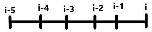
Based on the calculated number of nodes, the formulated equation would be,
Hypothesis equation= `Deltax^2*(d^2u)/dx^2=a*f(i)+b*f(i-1)+c*f(i-2)+d*f(i-3)+e*f(i-4)+g*f(i-5)`

Taylor expansion of the terms in the equations:

`a*f(i)=a*f(i)`

`b*f(i-1)=b(f(i)-Deltaxf(i)+(Deltax^2)/(2!)f(i)-(Deltax^3)/(3!)f(i)+(Deltax^4)/(4!)f(i)-(Deltax^5)/(5!)f(i))`

`c*f(i-2)=c(f(i)-2Deltaxf(i)+(2Deltax)^2/(2!)f(i)-(2Deltax)^3/(3!)f(i)+(2Deltax)^4/(4!)f(i)- (2Deltax)^5/(5!)f(i))`

`d*f(i-3)=d(f(i)-3Deltaxf(i)+(3Deltax)^2/(2!)f(i)-(3Deltax)^3/(3!)f(i)+(3Deltax)^4/(4!)f(i)- (3Deltax)^5/(5!)f(i))`

`e*f(i-4)=e(f(i)-4Deltaxf(i)+(4Deltax)^2/(2!)f(i)-(4Deltax)^3/(3!)f(i)+(4Deltax)^4/(4!)f(i)- (4Deltax)^5/(5!)f(i))`

`g*f(i-5)=g(f(i)-5Deltaxf(i)+(5Deltax)^2/(2!)f(i)-(5Deltax)^3/(3!)f(i)+(5Deltax)^4/(4!)f(i)- (5Deltax)^5/(5!)f(i))`

Taylor Table:

`Stencils darr`

Taylor series expansion `rarr`

`Deltax^2 * (d^2u)/dx^2`	f(i)	`Deltaxf'(i)`	`Deltax^2 f''(i)`	`Deltax^3 f'''(i)`	`Deltax^4 f''''(i)`	`Deltax^5 f'''''(i)`
`a*f(i)`	a	0	0	0	0	0
`b*f(i-1)`	b	-b	`b/2`	`-b/6`	`b/24`	`-b/120`
`c*f(i-2)`	c	-2c	`(4*c)/2`	`-(8*c)/6`	`(16*c)/24`	`-(32*c)/120`
`d*f(i-3)`	d	-3d	`(9*d)/2`	`-(27*d)/6`	`(81*d)/24`	`-(243*d)/120`
`e*f(i-4)`	e	-4e	`(16*e)/2`	`-(64*e)/6`	`(256*e)/24`	`-(1024*e)/120`
`g*f(i-5)`	g	-5g	`(25*g)/2`	`-(125*g)/6`	`(625*g)/24`	`-(3125*g)/120`
`sum`	0	0	1	0	0	~0

We will equate the following equations and get values of the variable. Five variables, first first equations.

`(a+b+c+d+e+g) = 0` ............ (1)

`(-b-2c-3d-4e-5g) = 0` .............(2)

`(b+4c+9d+16e+25g)/2 = 1` ......... (3)

`(-b-8c-27d-64e-125g)/6 = 0` ............(4)

`(b+16c+81d+256e+625g)/24 = 0` ......... (5)

`(-b-32c-243d-1024e-3125g)/120 = 0` .......(6)

Thus the coefficient values are:
a = 3.7500
b = -12.8333
c = 17.8333
d = -13.0000
e = 5.0833
g = -0.8333

Upon calculating we obtained the variable values and thus, putting them in hypothesis equation:

`=>Deltax^2*(d^2u)/dx^2=3.7500*f(i)-12.8333*f(i-1)+17.8333*f(i-2)-13*f(i-3)+5.0833*f(i-4)-0.8333*f(i-5)`

• Central difference:

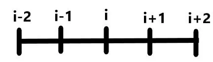
Based on the calculated number of nodes, the formulated equation would be,
Hypothesis equation = `Deltax^2*(d^2u)/dx^2=a*f(i-2)+b*f(i-1)+c*f(i)+d*f(i+1)+e*f(i+2)`

Taylor expansion of the terms in the equation:

`a*f(i-2)=a(f(i)-2Deltaxf(i)+(2Deltax)^2/(2!)f(i)-(2Deltax)^3/(3!)f(i)+(2Deltax)^4/(4!)f(i))`

`b*f(i-1)=b(f(i)-Deltaxf(i)+(Deltax)^2/(2!)f(i)-(Deltax)^3/(3!)f(i)+(Deltax)^4/(4!)f(i))`

`c*f(i) = c*f(i)`

`d*f(i+1)=d(f(i)+Deltaxf(i)+(Deltax^2)/(2!)f(i)+(Deltax^3)/(3!)f(i)+(Deltax^4)/(4!)f(i))`

`e*f(i+2)=e(f(i)+2Deltaxf(i)+(2Deltax)^2/(2!)f(i)+(2Deltax)^3/(3!)f(i)+(2Deltax)^4/(4!)f(i))`

Taylor Table:

`Stencils darr`

Taylor series expansion `rarr`

`Deltax^2 * (d^2u)/dx^2`	f(i)	`Deltaxf'(i)`	`Deltax^2 f''(i)`	`Deltax^3 f'''(i)`	`Deltax^4 f''''(i)`
`a*f(i-2)`	a	-2a	`(4*a)/2`	`-(8*a)/6`	`(16*a)/24`
`b*f(i-1)`	b	-b	`b/2`	`-b/6`	`b/24`
`c*f(i)`	c	0	0	0	0
`d*f(i+1)`	d	d	`(d)/2`	`(d)/6`	`(d)/24`
`e*f(i+2)`	e	2e	`(4*e)/2`	`(8*e)/6`	`(16*e)/24`
`sum`	0	0	1	0	0

We will equate the following equations and get values of the variable.

`(a+b+c+d+e) = 0` ............ (1)

`(-2a-b+d+2e) = 0` .............(2)

`(4a+b+d+4e)/2 = 1` ......... (3)

`(-8a-b+d+8e)/6 = 0` ............(4)

`(16a+b+d+16e)/24 = 0` ......... (5)

Thus the coefficient values are:
a = -0.0833
b = 1.3333
c = -2.5000
d = 1.3333
e = -0.0833

Upon calculating we obtained the variable values and thus, putting them in hypothesis equation:

`=>Deltax^2*(d^2u)/dx^2=-0.0833*f(i-2)+1.3333*f(i-1)-2.5*f(i)+1.3333*f(i+1)-0.0833*f(i+2)`

• Proving Skewed scheme is of fourth-order approximation:

Given Formula:
The order of accuracy P = Number of nodes in the stencil N - order of derivative Q for one-sided/skewed schemes

Here, N = 6, Q = 2 `=> P= N-Q = 4`

Thus we know it is, skewed scheme of fourth-order accuracy.

• MATLAB CODE:

MAIN CODE:

%Defining x and dx
x=pi/3;
dx=linspace(pi/400,pi/40,20);

%Finding Coefficients using the matrix form:
%Solved using matrix inversion method.
%Skewed Right Sided Difference Coefficients:
A1=[1,1,1,1,1,1;0,1,2,3,4,5;0,1/2,4/2,9/2,16/2,25/2;0,1/6,8/6,27/6,64/6,125/6;0,1/24,16/24,81/24,256/24,625/24;
    0,1/120,32/120,243/120,1024/120,3125/120];
B1=[0;0;1;0;0;0]; %Sum values of the equations
X = inv(A1)*B1

%Skewed Left Sided Difference Coefficients
A2=[1,1,1,1,1,1;0,-1,-2,-3,-4,-5;0,1/2,4/2,9/2,16/2,25/2;0,-1/6,-8/6,-27/6,-64/6,-125/6;0,1/24,16/24,81/24,256/24,625/24;
    0,-1/120,-32/120,-243/120,-1024/120,-3125/120];
B2=[0;0;1;0;0;0];%Sum values of the equations
Y = inv(A2)*B2

%Central Difference Coefficients
A3=[1,1,1,1,1;-2,-1,0,1,2;4/2,1/2,0,1/2,4/2;-8/6,-1/6,0,1/6,8/6; 16/24,1/24,0,1/24,16/24];
B3=[0;0;1;0;0]; %Sum values of the equations
Z = inv(A3)*B3

%Finding Error
for i=1:length(dx)
    error_skewed_right_sided(i)=Skewed_Right_Sided(x,dx(i),X);
    error_skewed_left_sided(i)=Skewed_Left_Sided(x,dx(i),Y);
    error_central(i)=Central(x,dx(i),Z);
    error_forward_difference(i)= forward_difference(x,dx(i));
    error_backward_difference(i)= backward_difference(x,dx(i));
end

%Plotting
figure(1)
loglog(dx,error_skewed_right_sided,'k')
hold on
loglog(dx,error_skewed_left_sided,'m')
hold on
loglog(dx,error_central,'g')
hold on 
loglog(dx,error_forward_difference,'c')
hold on 
loglog(dx,error_backward_difference,'rd')

grid on

legend('Skewed Right Sided','Skewed Left Sided','Central','Forward Difference','Backward Difference') 
xlabel('Value of dx')
ylabel('Error')

Analytical function:

%Solving for Analytical function = exp(x)*cos(x)
function output = a_f(x)
output = exp(x)*cos(x);
end

Right-Sided Differential function:

function error = Skewed_Right_Sided(x,dx,X)
analytical_derivative =f''(x) -2*exp(x)*sin(x);

%Numerical derivative of Skewed_Right_Sided:
Skewed_Right_Sided_der = (X(1)*a_f(x)+X(2)*a_f(x+dx)+X(3)*a_f(x+(2*dx))+X(4)*a_f(x+(3*dx))+X(5)*a_f(x+(4*dx))+X(6)*a_f(x+(5*dx)))/(dx)^2
error = abs(Skewed_Right_Sided_der - analytical_derivative)
end

Left-Sided Differential function:

function error = Skewed_Left_Sided(x,dx,X)
analytical_derivative = -2*exp(x)*sin(x);

%Numerical derivative Skewed_Left_Sided:
Skewed_Left_Sided_der = (X(1)*a_f(x)+X(2)*a_f(x-dx)+X(3)*a_f(x-(2*dx))+X(4)*a_f(x-(3*dx))+X(5)*a_f(x-(4*dx))+X(6)*a_f(x-(5*dx)))/(dx)^2
error = abs(Skewed_Left_Sided_der - analytical_derivative)
end

Central Differential function:

function error = Central(x,dx,X)
analytical_derivative = -2*exp(x)*sin(x);

%Numerical derivative Central:
Central_der = (X(1)*a_f(x-(2*dx))+X(2)*a_f(x-dx)+X(3)*a_f(x)+X(4)*a_f(x+dx)+X(5)*a_f(x+(2*dx)))/(dx)^2
error = abs(Central_der - analytical_derivative)
end

Forward Differential function:

function error = forward_difference(x,dx)
analytical_derivative = -2*exp(x)*sin(x);
%Numerical derivative forward difference:
 forward_difference = ((exp(x+dx)*cos(x+dx))-(exp(x)*cos(x)))/dx;
 error=abs(forward_difference- analytical_derivative);
end

Backward Differential function:

function error = backward_difference(x,dx)
analytical_derivative = -2*exp(x)*sin(x);
%Numerical derivative forward difference:
backward_difference = ((exp(x)*cos(x))-(exp(x-dx)*cos(x-dx)))/dx;
error=abs(backward_difference- analytical_derivative);
end

Error-values and Graph:

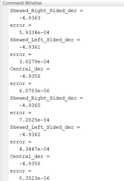
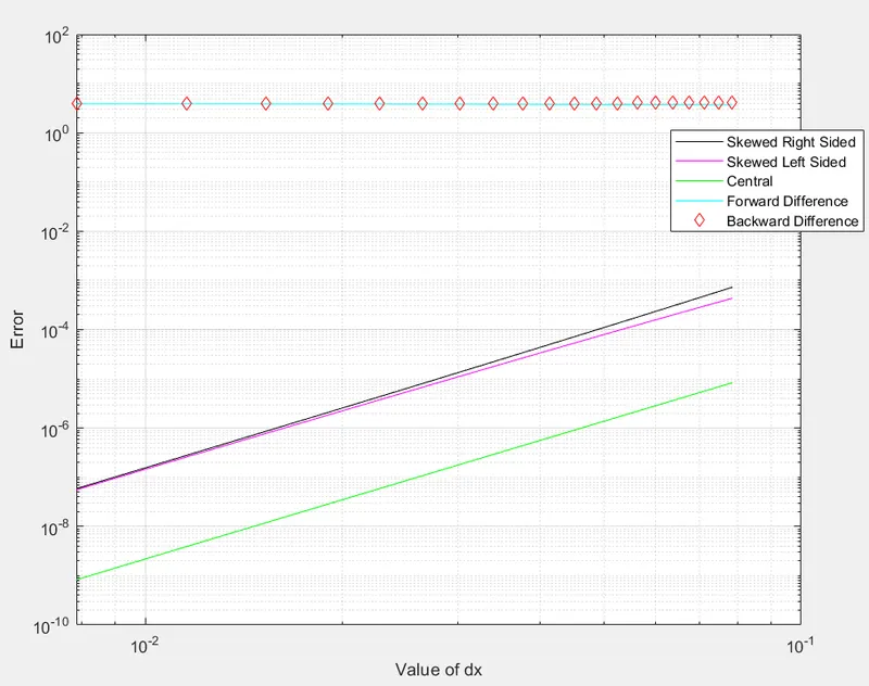
Code Explanation:

• Using the matrix form, we have calculated the values of coefficients for the Left, Right and Central differential equations. As the values for matrix A and B are defined, the matrix X, consisting of the unknowns, a, b, c, d, e and g, can be evaluated using the inversion formula, `X=A^(−1)B`
• We have made individual function codes for all the differentials and called all the functions in the main function where we are using it for making an error plot.
• We have used for-loop in the program to repeatedly run the program to get the different error terms and plot them for evaluation. The loop runs 20 times, giving us 20 different values of all the differential terms.
• Error is the absolute difference between the side differential and the analytical derivative of the given function.

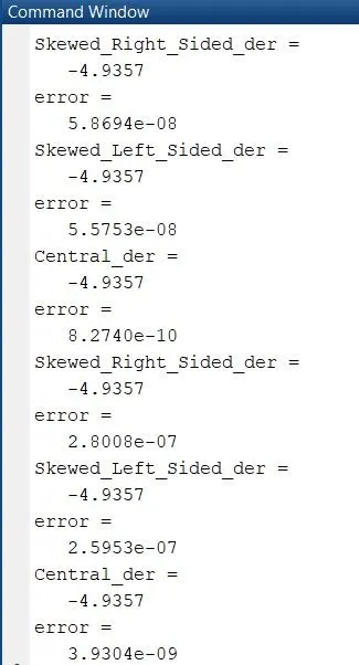
Result: We can understand the difference in the error values between all three types of derived differentials. The left and right side differentials have close values for the error and increase w.r.t dx, while the central derivative shows the least values of error out of all three. Since forward and backward approximations are of second-order error, they give out larger errors than the other fourth-order schemes. Error at higher-order schemes is bigger than that of the lower order schemes. This is due to higher roundoff errors at those points. That's why we have used the values of x and dx in fractional form instead of decimal to avoid this roundoff error.

We can clearly see the straight-line graph of forward and backward difference. Their value of the error doesn't vary with dx, hence higher error is observed in forward and backward schemes due to a lesser number of data points being used for calculation when compared to other schemes.

Central Derivative error < Left Skewed Derivative < Right Skewed Derivative

Advantages of the Skewed scheme over Central Difference scheme:

• If the flow is from left to right, then a skewed left-sided scheme is used; else if the flow is from right to left, a skewed right-sided scheme is employed. The skewed scheme needs only one direction for calculation but the CD scheme needs both the side values and thus causes a problem in some instances.
• While a skewed scheme is significant in this application; a central scheme is used in cases where diffusion takes place and the data from all directions are required to compute the values.
• Skewed schemes have higher accuracy than CD schemes.
• If we want to calculate single or higher-order derivatives at the corner node CD scheme can't be used at that moment.