Discretization over a range for a simple function using different orders of approximation

The first part of the Question had already been computed the single value of first, second and fourth-order of approximation for the given value of x and dx. In this, we will compute the same, for a wider range and obtain multiple discrete values for the given function.

Given: Analytical function: `f(x) = sin(x)/x^3`

`x = pi/3`, dx ranges from `[pi/4000,pi/40,20]`, with 20 as number of terms to be calculated between `pi/4000 & pi/40` as upper and lower limit for the iteration.

Program Explanation:

In this program, we have calculated the first, second and fourth-order of derivatives for all the given values of dx at x=`pi/3`.
The problem is solved using the external function method, in which, sections of the problems are solved separately and then called into the main program command. In this, separate files for calculation first, second and fourth-order approximation were created and then called into another file with the main function in it to plot the graphs and merge the data.

The formula for order approximation calculation:
First Order approximation or forward differencing = `(f(x+dx) + f(x)) /dx`
Second-Order approximation or central differencing = `(f(x+a)-F(x-a))/(2*dx)`
Fourth-Order approximation or differencing = `(f ( x − 2 ⋅ d x ) − ( 8 ⋅ f ( x − d x ) ) + ( 8 ⋅ f ( x + d x ) ) − f ( x + 2 ⋅ d x ))/ (12 ⋅ d x)`

Formula for slope calculation:

Slope = difference in absolute error(in log10)./difference in dx(in log10)

• A first-order approximation is calculated in a file named, "first_order".
• A second-order approximation is calculated in a file named, "second_order".
• A fourth-order approximation is calculated in a file named, "fourth_order".

These three files won't show any output as values of x and dx are not provided in them. It will show an error when that program is run independently. (the error is shown below)

• After writing these files, all are called in the main file under for loop, section to get different values of approximations.
• Then this program is run and won't show any error as this file defines the input values for the attached files. There all the calculations are done and send back to the main file for executing the plotting commands.
• These error values are then placed in graph using two types of format:
  'Plot' and 'Log-log'.
• Two graphs are plotted to observe the curve patter to get brief insight of the error pattern.
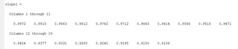
• Lastly, the slope for log graph is calculted to observe the drastic decrease in error values more clearly as the order increases.

Program:

• Main Code:
  Code connecting the first, second and fourth-order of approximation functions and plotting:

clear all
close all
clc

% inputs for program:
x = pi/3;
dx = linspace(pi/4000,pi/40,20); % dx is the range for the derivative 
% analytical function f(x) = sin(x)/x^3
% analytical term's derivative f'(x): 
analytical_derivative = ((x^3*(cos(x)))- (sin(x)*(3*(x^2))))/(x^6);

%Preallocation of the absolute errors(Initiallization):
for i = 1:length(dx)
    error_first_order(i)= first_order(x,dx(i)); % calling the function for calculating 1st order error
   error_second_order(i)= second_order(x,dx(i)); % calling the function for calculating 2nd order error
    error_fourth_order(i)= fourth_order(x,dx(i)); % calling the function for calculating 4th order error    
end
%Plotting:
figure(1)
plot(dx,error_first_order,'m','linewidth',2)
hold on 
plot(dx,error_second_order,'y','linewidth',2)
hold on
plot(dx,error_fourth_order,'x-','linewidth',2)
legend('First order Error', 'Second order Error', 'Fourth order Error')
xlabel('dx')
ylabel('Absoulte error terms')
title('Plot of dx v/s order approximation error terms')
grid on

% Getting values of different order of approximation to get the linear
% values in one graph.
figure(2)
loglog(dx,error_first_order)
hold on
loglog(dx,error_second_order)
hold on
loglog(dx, error_fourth_order)
legend('First order Error', 'Second order Error', 'Fourth order Error')
xlabel('dx')
ylabel('Absoulte error terms')
title('dx v/s 1st, 2nd and 4th order approximation error')
grid on

% To get the slope of the loglog curves, and so the error and dx values are converted into log terms:
slope1 = diff(log10(error_first_order))./diff(log10(dx))
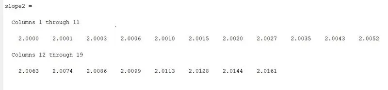
slope2 = diff(log10(error_second_order))./diff(log10(dx))
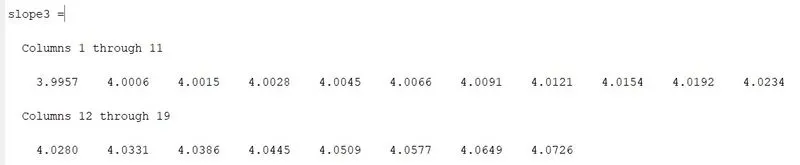
slope3 = diff(log10(error_fourth_order))./diff(log10(dx))

• Function Codes:
  Code for calculating First order of approximation:

function error =  first_order(x,dx)
analytical_derivative = ((x^3*(cos(x)))- (sin(x)*(3*(x^2))))/(x^6);
 forward_difference = ((sin(x+dx)/(x+dx)^3)-(sin(x)/(x)^3))/dx;
 error=abs(forward_difference- analytical_derivative);
end

Code for calculating Second order of approximation:

function error =  second_order(x,dx)
analytical_derivative = ((x^3*(cos(x)))- (sin(x)*(3*(x^2))))/(x^6);
 central_difference = ((sin(x+dx)/(x+dx)^3)-(sin(x-dx)/(x-dx)^3))/(2*dx);
 error = abs(central_difference - analytical_derivative);
end​

Code for calculating Fourth order of approximation:

function error =   fourth_order(x,dx)
analytical_derivative = ((x^3*(cos(x)))- (sin(x)*(3*(x^2))))/(x^6);
 differencing = (((sin(x-2*dx)/(x-2*dx)^3) - 8*(sin(x-dx)/(x-dx)^3)+ 8*(sin(x+dx)/(x+dx)^3)- (sin(x+2*dx)/(x+2*dx)^3)))/(12*dx);
 error = abs(differencing - analytical_derivative);
end

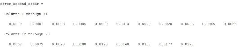
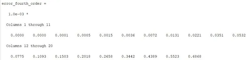
Obtained errors for observation of trend: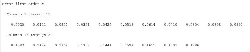

Graph and Slope Explanation:

• The proper labelling is done on the graphs to observe the obtained data.
  
  
• The slope for the three plots is positive since the line moves upward when moving from left to right.
• Slope also tells us the rate at which change takes place.
• For first-order error, the average slope of the curve is 0.9 when moving from left to right (when dx increases), rate of increase of absolute error is the least.
• For second-order error, the average slope of the curve is 2 the rate of increase of absolute error is greater than the first-order error but less than the fourth-order error.
• For fourth-order, the average slope of the curve is 4.0 when moving from left to right (when dx increases), the rate of increase of absolute error is highest.
  
  
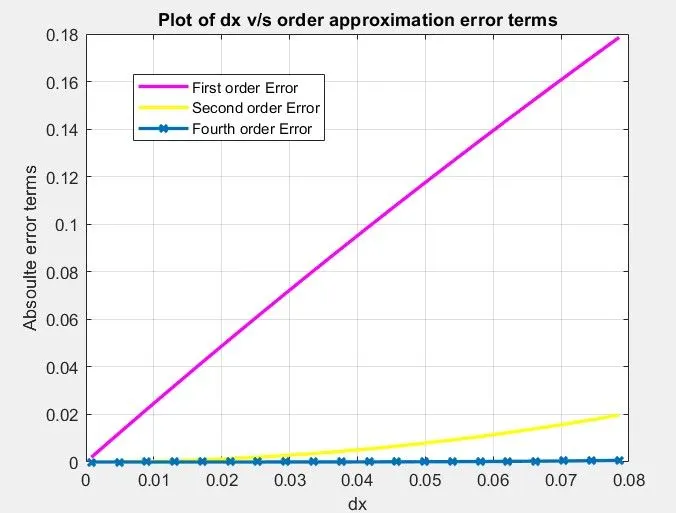
• From the above graph, we can clearly see that the value for error in 1st order, 2nd order and 4ht order approximation is decreasing as the value of dx is decreasing. The highest error value is for 1st order approximation, the 4th order error value being the lowest.

First-order error > Second order error > Fourth order error

Results:
Graph 1:

Graph 2:

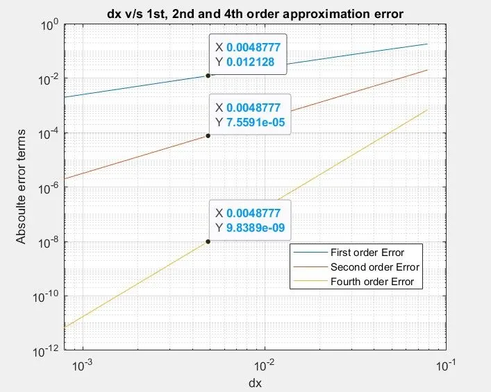
Graph 1 is made using plot command, in while the curves are not in the same order so can be a bit difficult to analyze the results while graph 2 is made using the log-log command while making all the curves to linear curves and thus much easier to analyze that obtained data.

Hence, we have met our objective successfully.