Damped Pendulum Oscillations

A pendulum is a weight suspended from a pivot so that it can swing freely. When a pendulum is displaced sideways from its resting(equilibrium) position. It continues to swing and gradually slows down due to the damping(resistance) effect on the body and will stop swinging at the equilibrium position where all the displacing forces are zero.

`(d^2theta)/(dt^2)+b/m(d theta)/dt + g/L(sin theta) = 0`

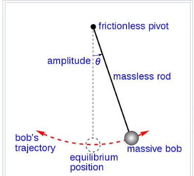
General ODE for a simple pendulum with damping where,

g = gravity in m/s2,

L = length of the pendulum in m,

m = mass of the ball in kg,

b=damping coefficient.

Given parameters to be used for calculation of ODE:

L=1 metre
m=1 kg
b=0.05
g=9.81 `m/s^2`.

Solving ODE: Since MATLAB can't solve ODE of higher-order we have to simplify the ODE into a simple first-order equation for computing. We'll assign higher-order terms to lower-order variables for computing and making the first-order equation.

Let's say, `theta = theta_1`
`(d theta)/dt = (d theta_1)/dt = theta_2` ...........`(color(green)(1))`

Now, `(d^2 theta_1)/dt^2 = (d theta_2)/dt` ............(`:.`2nd order term is converted to first order)...........`(color(green)(2))`

Now substitute equation (1) and (2) in the the general equation, thus we get:-

`(d theta_2)/dt + b/m theta_2 + g/L(sin theta_1)=0`

`=> (d theta_2)/dt = -b/m theta_2 - g/L(sin theta_1)..........(color(green)(3))`

`(d theta)/dt = [((d theta_1)/dt ), ((d theta_2)/dt)] => [((d theta_1)/dt ), ((d theta_2)/dt)]= [(theta_2),(-b/m theta_2-g/Lsintheta_1)]`

This equation will be used to calculate the displacement and angular momentum of pendulum.

MATLAB Code:

Main Code:

%Solving the final equation
%initial conditions
L=1;
t = [0 20];
theta_0=[0 3];
%solving ODE using external file named "odefun_derivative"
[t, theta] = ode45('odefun_derivative',t,theta_0);
% other format to write ode is using annanomous function:
%[t,results] = ode45(@(t,theta) odefun_derivative(t,theta,L,m,b,g), t,theta_0);

%plotting code to get graphs for pendulum oscillation.
figure(1)
plot(t, theta(:,1),'r','lineWidth',2);
hold on 
grid on
plot(t,theta(:,2),'m','lineWidth',2);
xlabel('Time(sec.)')
ylabel('Displacement and angular velocity')
legend('Displacement','angular velocity')
title('Displacement and angular velocity v/s. Time curve')
ct=1;
for i=1:length(t)
% initial condition for attaching pendulum to a surface.  
  x_initial=0;
    y_initial=0;
    x = L*sin(theta(i,1));
    y = -L*cos(theta(i,1));
   
    figure(2)
    plot(x,y,'o','markerfacecolor','r', 'markersize',10)
    hold on
    grid on
    plot(x_initial,y_initial,'k')
    hold on
    plot([x_initial,x],[y_initial,y],'g','lineWidth', 2)
    plot([-1 1],[0 0],'lineWidth',2) % attach surface line
    axis([-1.5 1.5 -2 2]) % Axis size
    title({'Damped Pendulum Oscillation', num2str(t(ct),'Time = %4.3f(sec)')})
    hold off;
    pause(0.05)
    M(ct)= getframe(gcf);
    ct=ct+1;
end
movie(M)
videofile = VideoWriter('Pendulum_oscillation.avi','Uncompressed AVI');
open(videofile)
writeVideo(videofile, M)
close(videofile)

Differential Function:

function [theta_dot]= odefun_derivative(t,theta)
%input values
L=1;
m=1;
b=0.05;
g=9.81;
theta_dot=zeros(2,1); % making a column matrix for placing differential terms
% first order derivative term
theta_dot(1)= theta(2); 
% secound order derivative term
theta_dot(2)= -(b/m)*theta(2)-(g/L)*sin(theta(1)); 
end

Output:

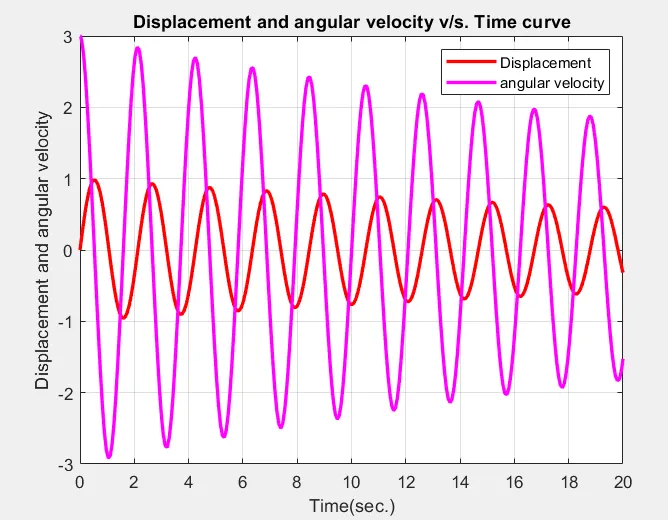
Video Link:
https://youtu.be/9qwu121hbqo