DERIVING 4th ORDER APPROXIMATION OF 2nd ORDER DERIVATIVE USING TAYLOT TABLE METHOD

AIM : To derive the following 4th order approximations scheme of the second order derivative:

OBJECTIVE :

-To write a program in MATLAB to evaluate the second order derivative of the analytical function,

i.e. `f(x) = e^x × cos.x` and comparing it with the 3 numerical approximations.
-Plot, compare the absolute error with respect to above mentioned schemes.
1. Central Difference
2. Skewed Right Sided Difference
3. Skewed Left Sided difference

-Comparing above schemes with Forward and Backward Differencing approximation schemes.

PROCEDURE :

(1). Symmetric Central Difference Scheme

The number of Nodes required for 4th order approximation of a second-order derivative can be given by the equation-

N=P+Q-1 ; Where

N is the number of node.

Q is the order of derivative.

P is the order of the approximation.

Therefore, Number of nodes=4+2-1 ; N=5

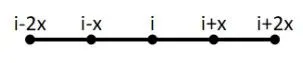
Consider the value of `(del^2y)/(del x^2)`with the 4th order of approximation is given by the equation

`(del^2y)/(del x^2) = (af(i-2)+bf(i-1) +cf(i)+df(i+1)+ef(i+2))/(Delta x^2`

Now, using taylor series to find the values of discrete poits with repect to point `i`

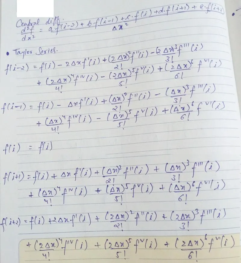
TAYLOR TABLE
		Taylor Series
		`f(i)`	`f'Deltax(i)`	`f''Deltax^2(i)`	`f'''Deltax^3(i)`	`f''''Deltax^4(i)`
Stencil	`af(i-2)`	`a`	`-2a`	`(4a)/2`	`(-8a)/6`	`(16a)/24`
	`bf(i-1)`	`b`	`-b`	`b/2`	`-b/6`	`b/24`
	`cf(i)`	`c`	`0`	`0`	`0`	`0`
	`df(i+1)`	`d`	`d`	`d/2`	`d/6`	`d/24`
	`ef(i+2)`	`e`	`2e`	`(4e)/2`	`(8e)/6`	`(16e)/24`
Sum of Coefficient		`0`	`0`	`1`	`0`	`0`

(2). Skewed 2nd Order Left-sided Difference Scheme

The number of Nodes required for 4th order approximation of a second-order derivative can be given by the equation-

N=P+Q ; Where

N is the number of node.

Q is the order of derivative.

P is the order of the approximation.

Therefore, Number of nodes=4+2 ; N=6

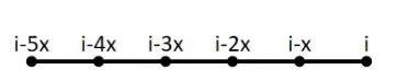
Consider the value of `(del^2y)/(del x^2)`with the 4th order of approximation is given by the equation

`(del^2y)/(del x^2) = (af(i)+bf(i-1) +cf(i-2)+df(i-3)+ef(i-4)+gf(i-5))/(Delta x^2`

Now, using taylor series to find the values of discrete poits with repect to point `i`

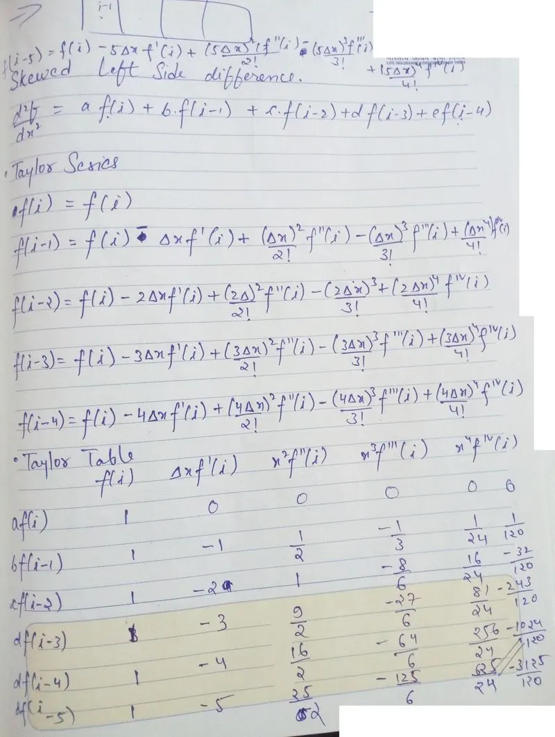
TAYLOR TABLE
		Taylor Series
		`f(i)`	`f'Deltax(i)`	`f''Deltax^2(i)`	`f'''Deltax^3(i)`	`f''''Deltax^4(i)`	`f'''''Deltax^5(i)`
Stencil	`af(i)`	`a`	`0`	`0`	`0`	`0`	`0`
	`bf(i-1)`	`b`	`-b`	`b/2`	`-b/6`	`b/24`	`-b/120`
	`cf(i-2)`	`c`	`-2c`	`c`	`(-8c)/6`	`(26c)/24`	`(-32c)/120`
	`df(i-3)`	`d`	`-3d`	`(9d)/2`	`(-27d)/6`	`(81d)/24`	`(-243d)/120`
	`ef(i-4)`	`e`	`-4e`	`(16e)/2`	`(-64e)/6`	`(256e)/24`	`(-1024e)/120`
	`gf(i-5)`	`g`	`-5g`	`(25g)/2`	`(-125g)/6`	`(625g)/24`	`(-3125g)/120`
Sum of Coefficient		`0`	`0`	`1`	`0`	`0`	`0`

(3). Skewed 2nd Order Reight-sided Difference Scheme

The number of Nodes required for 4th order approximation of a second-order derivative can be given by the equation-

N=P+Q ; Where

N is the number of node.

Q is the order of derivative.

P is the order of the approximation.

Therefore, Number of nodes=4+2 ; N=6

Consider the value of `(del^2y)/(del x^2)`with the 4th order of approximation is given by the equation

`(del^2y)/(del x^2) = (af(i)+bf(i+1) +cf(i+2)+df(i+3)+ef(i+4)+gf(i+5))/(Delta x^2`

Now, using taylor series to find the values of discrete poits with repect to point `i`

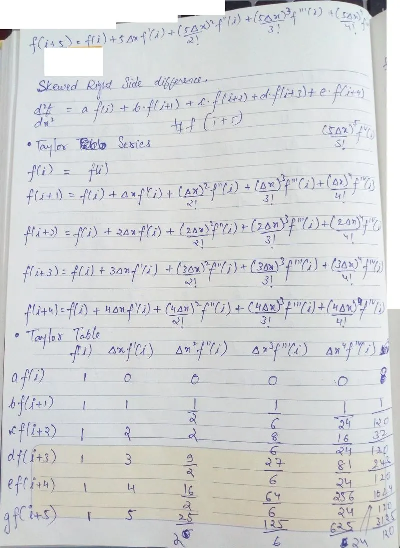
TAYLOR TABLE
		Taylor Series
		`f(i)`	`f'Deltax(i)`	`f''Deltax^2(i)`	`f'''Deltax^3(i)`	`f''''Deltax^4(i)`	`f'''''Deltax^5(i)`
Stencil	`af(i)`	`a`	`0`	`0`	`0`	`0`	`0`
	`bf(i+1)`	`b`	`b`	`b/2`	`b/6`	`b/24`	`b/120`
	`cf(i+2)`	`c`	`2c`	`c`	`(8c)/6`	`(26c)/24`	`(32c)/120`
	`df(i+3)`	`d`	`3d`	`(9d)/2`	`(27d)/6`	`(81d)/24`	`(243d)/120`
	`ef(i+4)`	`e`	`4e`	`(16e)/2`	`(64e)/6`	`(256e)/24`	`(1024e)/120`
	`gf(i+5)`	`g`	`5g`	`(25g)/2`	`(125g)/6`	`(625g)/24`	`(3125g)/120`
Sum of Coefficient		`0`	`0`	`1`	`0`	`0`	`0`

TAYLOR TABLE METHOD MAIN PROGRAM :

clear all
close all
clc

x=pi/3;

dx=linspace(pi/4,pi/400,80);

%Analytical_derivative of Function=exp(x)*cos(x);

%Second_order_analytical_derivative;
analytical_derivative=-2*exp(x)*sin(x);

%central differencing(4th order approimation)
%Solving for the coefficients
A=[1, 1, 1, 1, 1;-2, -1, 0, 1, 2;4/2, 1/2, 0, 1/2, 4/2;-8/6, -1/6, 0, 1/6, 8/6;16/24, 1/24, 0, 1/24, 16/24];
B=[0;0;1;0;0];
x_c=inv(A)*B;

%Skewed left-sided(4th order approimation)
%Solving for the coefficients
C=[1 1 1 1 1 1;0 -1 -2 -3 -4 -5;0 1/2 4/2 9/2 16/2 25/2;0 -1/6 -8/6 -27/6 -64/6 -125/6;0 1/24 16/24 81/24 256/24 625/24;0 -1/120 -32/120 -243/120 -1024/120 -3125/120];
D=[0;0;1;0;0;0];
x_l=inv(C)*D;

%Skewed right-sided(4th order approimation)
%Solving for the coefficients
E=[1 1 1 1 1 1;0 1 2 3 4 5;0 1/2 4/2 9/2 16/2 25/2;0 1/6 8/6 27/6 64/6 125/6;0 1/24 16/24 81/24 256/24 625/24;0 1/120 32/120 243/120 1024/120 3125/120];
F=[0;0;1;0;0;0];
x_r=inv(E)*F;
 
%numerical derivative

central_difference=((x_c(1).*exp(x-2.*dx).*cos(x-2.*dx))+(x_c(2).*exp(x-dx).*cos(x-dx))+(x_c(3).*exp(x).*cos(x))+(x_c(4).*exp(x+dx).*cos(x+dx))+(x_c(5).*exp(x+2.*dx).*cos(x+2.*dx)))./(dx.^2); 

left_difference=((x_l(1).*exp(x).*cos(x))+(x_l(2).*exp(x-dx).*cos(x-dx))+(x_l(3).*exp(x-2.*dx).*cos(x-2.*dx))+(x_l(4).*exp(x-3.*dx).*cos(x-3.*dx))+(x_l(5).*exp(x-4.*dx).*cos(x-4.*dx))+(x_l(6).*exp(x-5.*dx).*cos(x-5.*dx)))./(dx.^2);
 
right_difference=((x_r(1).*exp(x).*cos(x))+(x_r(2).*exp(x+1.*dx).*cos(x+1.*dx))+(x_r(3).*exp(x+2.*dx).*cos(x+2.*dx))+(x_r(4).*exp(x+3.*dx).*cos(x+3.*dx))+(x_r(5).*exp(x+4.*dx).*cos(x+4.*dx))+(x_r(6).*exp(x+5.*dx).*cos(x+5.*dx)))./(dx.^2);
 
%absolute error
error_c=abs(analytical_derivative-central_difference); 
error_l=abs(analytical_derivative-left_difference);
error_r=abs(analytical_derivative-right_difference);
error=[error_c;error_l;error_r];
 
figure(1)
loglog(dx,error_c,'g') 
hold on
loglog(dx,error_l,'b')
loglog(dx,error_r,'r')
title('Error Curves')
ylabel('Absolute Error')
xlabel('Grid Spacing(dx)')
legend('Central Differencing','Left Differencing','Right Differencing')

PLOT :

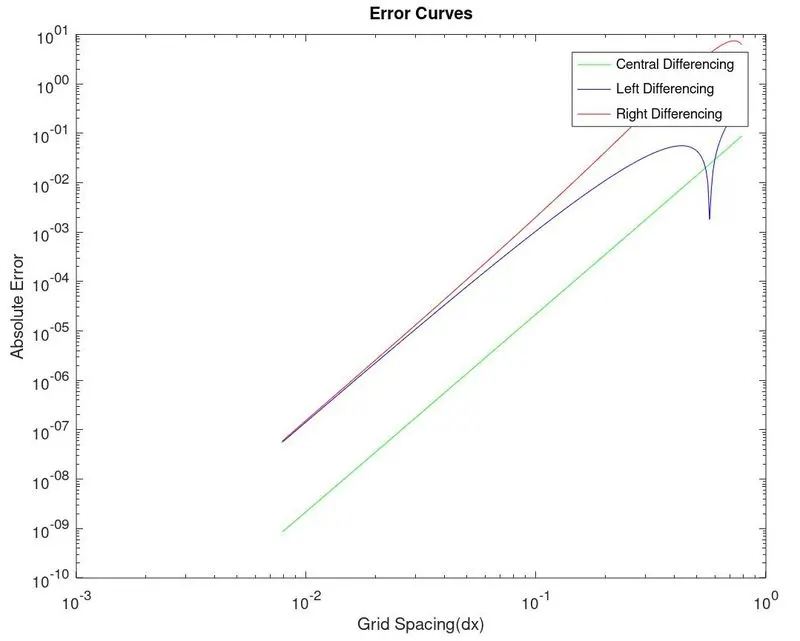
CONCLUSION :

• As we can see from the above figure the error for the central difference method is very less compared to the skewed methods.
• Skewed right and left difference methods almost gives the same results in terms of error for a small value of time step.
• When data from the grid points is only available from either the left or right end i.e. at nodes closer to the boundaries,for computations that requires a high order approximations we make use of skewed schemes.
• For better consistency of scheme to be maintained the values of dx are kept as low as possible for providing proper computational plots.