Week 3.5 - Deriving 4th order approximation of a 2nd order derivative using Taylor Table method

Aim:

To derive equations for 4th order approximations of the second-order derivative by using methods i.e. Central difference, Skewed right-sided difference, Skewed left-sided difference and to evaluate the results from MATLAB program for the given methods with the help of Taylor's table.

Theory:

Central difference method

For any finite difference method, one needs to define an order of accuracy. For central schemes, following expression is used,

Order of accuracy P = Number of nodes in the stencil N - Order of derivative Q + 1

To get an order of accuracy of 4, provided with 2nd order of derivative, we need to take 5 nodes on the stencil. Following stencil gives an idea about nodes to be taken,

An expression for 2nd order derivative having 4th order approximation is,

`(del^2f)/(delx^2)= (a*f_(i-2)+b*f_(i-1)+c*f_i+d*f_(i+1)+e*f_(i+2))/(Deltax^2)`

The coefficients a, b, c, d, e, are evaluated using Taylor's table. The function for this, is explained in following text.

Skewed left-sided difference method

Expression for order of accuracy for one-sided/skewed schemes, is given as follows,

Order of accuracy P = Number of nodes in the stencil N - Order of derivative Q

To get an order of accuracy of 4, provided with 2nd order of derivative, we need to take 6 nodes on the stencil. Following stencil gives an idea about nodes to be taken,

An expression for 2nd order derivative having 4th order approximation is,

`(del^2f)/(delx^2)= (a*f_(i)+b*f_(i-1)+c*f_(i-2)+d*f_(i-3)+e*f_(i-4)+f*f_(i-5))/(Deltax^2)`

The coefficients a, b, c, d, e, f, are evaluated using Taylor's table. The function for this, is explained in following text.

Skewed right-sided difference method

The order of accuracy will be same as that for previous method. Following stencil gives an idea about nodes to be taken,

An expression for 2nd order derivative having 4th order approximation is,

`(del^2f)/(delx^2)= (a*f_(i)+b*f_(i+1)+c*f_(i+2)+d*f_(i+3)+e*f_(i+4)+f*f_(i+5))/(Deltax^2)`

The coefficients a, b, c, d, e, f, are evaluated using Taylor's table. The function for this, is explained in following text.

Objectives:

• To write a program in Matlab to evaluate the second-order derivative of the analytical function 'exp(x)*cos(x)'
• To compare the second-order derivative with the 3 numerical approximations (explained earlier)
• To draw a plot that compares the absolute error between the above-mentioned schemes

MATLAB Program:

Central difference method function

function error_FROA_central=appr_central_difference(x,dx)
%Central diference approximation of 2nd order derivative
%Function exp(x)*cos(x)
analytical_second_order_derivative=-2*sin(x)*exp(x);

LHS=[1 1 1 1 1;-2 -1 0 1 2;4/2 1/2 0 1/2 4/2;-8/6 -1/6 0 1/6 8/6;16/24 1/24 0 1/24 16/24];
RHS=[0;0;1;0;0];
solution_central=inv(LHS)*RHS;
format rat
coefficients=(solution_central).';
a=coefficients(1);
b=coefficients(2);
c=coefficients(3);
d=coefficients(4);
e=coefficients(5);

fourth_order_approximation_central=(a*func(x-(2*dx))+b*func(x-dx)+c*func(x)+d*func(x+dx)+e*func(x+(2*dx)))/dx^2;

error_FROA_central=abs(analytical_second_order_derivative-fourth_order_approximation_central);
end

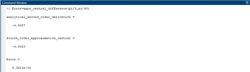
As explained earlier, the coefficients of 2nd order derivative expression using central scheme, are derived using Taylor's table. Taylor's table gives system of algebric equations, which can be solved by using matrix inversion method. 'LHS' consists of coefficients and 'RHS' consists of values of equations. Analytical derivative can be evaluated using an expression shown in above code. 'format rat' keeps the coefficients in fraction form. Absolute error can be found by using 'abs' command.

Skewed right-sided difference method function

function error_FROA_right_skewed=appr_skewed_right_sided_difference(x,dx)
%Central diference approximation of 2nd order derivative
%Function exp(x)*cos(x)
analytical_second_order_derivative=-2*sin(x)*exp(x);

LHS=[1 1 1 1 1 1;0 1 2 3 4 5;0 1/2 2 9/2 8 25/2;0 1/6 4/3 9/2 32/3 125/6;0 1/24 2/3 27/8 32/3 625/24;0 1/120 32/120 243/120 1024/120 3125/120];
RHS=[0;0;1;0;0;0];
solution_right_skewed=inv(LHS)*RHS;
format rat
coefficients=(solution_right_skewed).';
a=coefficients(1);
b=coefficients(2);
c=coefficients(3);
d=coefficients(4);
e=coefficients(5);
f=coefficients(6);

fourth_order_approximation_right=(a*func(x)+b*func(x+dx)+c*func(x+(2*dx))+d*func(x+(3*dx))+e*func(x+(4*dx))+f*func(x+(5*dx)))/dx^2;

error_FROA_right_skewed=abs(analytical_second_order_derivative-fourth_order_approximation_right);
end

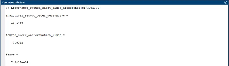
The code is similar to that for previous method. Only, the change is coefficients of skewed right-sided expression.

Skewed left-sided difference method function

function error_FROA_left_skewed=appr_skewed_left_sided_difference(x,dx)
%Central diference approximation of 2nd order derivative
%Function exp(x)*cos(x)
analytical_second_order_derivative=-2*sin(x)*exp(x);

LHS=[1 1 1 1 1 1;0 -1 -2 -3 -4 -5;0 1/2 2 9/2 8 25/2;0 -1/6 -4/3 -9/2 -32/3 -125/6;0 1/24 2/3 27/8 32/3 625/24;0 -1/120 -32/120 -243/120 -1024/120 -3125/120];
RHS=[0;0;1;0;0;0];
solution_left_skewed=inv(LHS)*RHS;
format short
coefficients=(solution_left_skewed).';
a=coefficients(1);
b=coefficients(2);
c=coefficients(3);
d=coefficients(4);
e=coefficients(5);
f=coefficients(6);

fourth_order_approximation_left=(a*func(x)+b*func(x-dx)+c*func(x-(2*dx))+d*func(x-(3*dx))+e*func(x-(4*dx))+f*func(x-(5*dx)))/dx^2;

error_FROA_left_skewed=abs(analytical_second_order_derivative-fourth_order_approximation_left);
end

The code is similar to that for previous method. Only, the change is coefficients of skewed left-sided expression.

Main program

clear all
close all
clc

%Inputs
x=pi/3;
dx=linspace(pi/4000,pi/40,20);

To plot 'dx' vs. 'Error', one needs range of 'dx'. This can done by using 'linspace' command. Value of 'x' is fixed i.e. x=pi/3.

%Looping
for i=1:length(dx)
    FROA_error_central(i)=appr_central_difference(x,dx(i));
    FROA_error_right(i)=appr_skewed_right_sided_difference(x,dx(i));
    FROA_error_left(i)=appr_skewed_left_sided_difference(x,dx(i));
end

For the length of 'dx', one has to calculate number of errors for respective methods. This can be done by looping. Here, 'for' loop runs the code for the length of 'dx' and stores the values in their respective arrays i.e FROA_error_central, FROA_error_right, FROA_error_left.

%Plotting
figure(1)
loglog(dx,FROA_error_central)
grid on
hold on
loglog(dx,FROA_error_right)
hold on
loglog(dx,FROA_error_left)
xlabel('dx')
ylabel('Error')
title('log plot of errors')
legend('Central difference error','Skewed right-sided difference error','Skewed left-sided difference error','location','southeast')

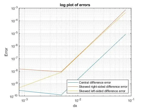
Here, 'loglog' command, creates as log plot, with values of 'dx' on x-axis and values of respective methods' errors on y-axis. 'figure' command creates a new figure window. 'xlabel, 'ylabel' are used for labelling. 'title' for titling the plot and 'legend' for respective method's error plot.

Outputs:

Central difference method function

#Result 1

#Result 2

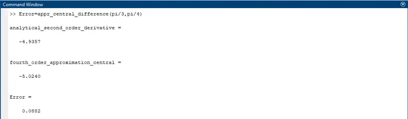
The above shown results are for different values of 'dx'. As 'dx' increases, the error increases. For central difference, this deviation is less.

Skewed right-sided difference method

#Result 1

#Result 2

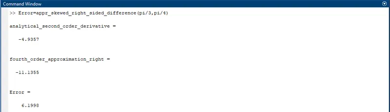
As compared to previous method, the deviation in two results is greater.

Skewed left-sided difference method

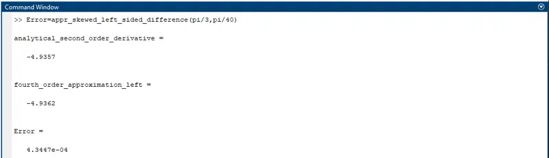
#Result 1

#Result 2

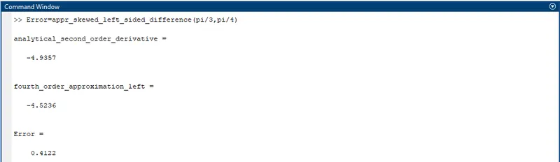
Error propagation is much less in this method as compared to skewed right-sided difference and slightly more as compared to central difference.

Error Plot for above-mensioned methods

Conclusion:

From plot, one can say that, the error is maximum for skewed right-sided difference approximation and minimum for central difference approximation. Error in skewed left-sided difference approximation is in between these two approximations.

When we compare central scheme with skewed schemes, the methodology for skewed schemes follows, values of derivative on either left side or right side. So, it does not depend on boundary conditions which is not the case for central scheme. This is advantageous in finding variables values at instant or at any space. Error might be more as compared to central scheme but to get an approximate result at higher rate, only be achieved with skewed schemes. From left-sided and right-sided schemes, prior is more accurate.