Week 3.2 - 2R Robotic Arm Challenge

Aim:

To develop a Matlab program to simulate the forward kinematics of a 2R Robotic Arm, as shown in the video.

Objective:

The objective of this challenge is to create a Matlab Program that simulates the forward kinematics of a 2R robotic arm. This requires computing the end-effector's position using input joint angles and arm lengths, which is then graphically visualized with Plots. The program will create an animation by assembling a series of frames depicting the arm's movement at various joint angles.

Approach:

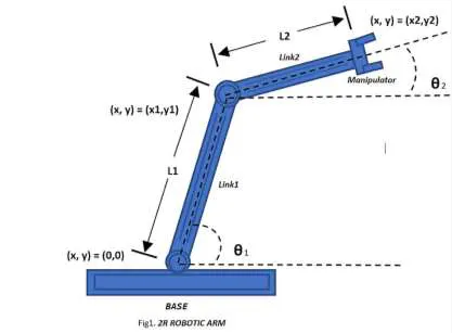
Figure 1: Forward kinematics of a 2R Robotic Arm.

A robotic arm, as depicted in Figure 1, is a type of mechanical arm that is typically programmable and can either be the full mechanism or a component of a more complex robot. These arms are made up of links that are joined by joints, allowing for rotational or linear motion. The links create a kinematic chain, with the terminal point known as the end effector. This effector, located at the arm's extremity, is meant to interact with the environment. Kinematic analysis examines the relationships between the manipulator's link locations, velocities, and accelerations. It is divided into two categories: direct kinematics and inverse kinematics. In forward kinematics, given the length of each link and the joint angle, the goal is to compute the position of any point within the robot's workspace. In inverse kinematics, link lengths and point position are used to determine joint angles. The research focuses on a 2R robotic arm with two rotational linkages that operate in a 2D plane, each with one degree of freedom.

Based on the dimensions shown in Figure 1, and using trigonometry:

𝑥0 = 𝑦0 = 0 (1)

𝑥1 = 𝐿1 cos 𝜃1 (2)

𝑦1 = 𝐿1 sin 𝜃1 (3)

𝑥2 = 𝑥1 + 𝐿2 cos 𝜃2 (4)

𝑦2 = 𝑦1 + 𝐿2 sin 𝜃2 (5)

The equations below represent the forward kinematics expressions for a two-link robotic arm. Trigonometric principles are used to determine the x and y coordinates of the arm's joints and end effector, taking into account the angles (θ₁ and θ₂) and link lengths (L₁ and L₂). The beginning position is at the origin, and succeeding positions are calculated by adding the horizontal and vertical parts of the link lengths, adjusting for the respective angles. These equations show a clear relationship between joint angles and the placements of robotic arm parts.

Matlab Program:

% Forward kinematics of a 2R Robotic Arm

% Define link lengths
L1 = 1; % Length of the first link (in meters)
L2 = 0.5; % Length of the second link (in meters)

% Define range of joint angles (in degrees)
theta1_range = linspace(0, 90, 10); % Range of theta1 values (adjust as needed)
theta2_range = linspace(0, 90, 10); % Range of theta2 values (adjust as needed)

% Convert angles from degrees to radians
theta1_rad = deg2rad(theta1_range); % Convert theta1 to radians
theta2_rad = deg2rad(theta2_range); % Convert theta2 to radians

% Initialize variables
x0 = 0; % Initial x-coordinate of the base
y0 = 0; % Initial y-coordinate of the base
num_frames = length(theta1_range) * length(theta2_range); % Total number of frames in the animation
X = zeros(num_frames, 1); % Initialize array to store x-coordinates of end-effector
Y = zeros(num_frames, 1); % Initialize array to store y-coordinates of end-effector

% Create video writer object for saving the animation
video = VideoWriter('forward_kinematics.avi'); % Create a VideoWriter object with filename 'forward_kinematics.avi'
video.FrameRate = 8; % Set the frame rate of the video (adjust as needed)
open(video); % Open the video writer object for writing frames

% Loop through all combinations of joint angles
frame = 1; % Initialize frame counter
for i = 1:length(theta1_rad) % Loop over theta1 values
  for j = 1:length(theta2_rad) % Loop over theta2 values
    % Calculate end-effector position using forward kinematics equations
    x1 = x0 + L1 * cos(theta1_rad(i)); % x-coordinate of the end of link 1
    y1 = y0 + L1 * sin(theta1_rad(i)); % y-coordinate of the end of link 1
    x2 = x1 + L2 * cos(theta2_rad(j)); % x-coordinate of the end-effector
    y2 = y1 + L2 * sin(theta2_rad(j)); % y-coordinate of the end-effector

    % Store end-effector coordinates
    X(frame) = x2; % Store x-coordinate of the end-effector
    Y(frame) = y2; % Store y-coordinate of the end-effector

    % Plot the robotic arm and end-effector
    plot([0 x1 x2], [0 y1 y2], 'o-', 'LineWidth', 2); % Plot the links and end-effector
    line([x0 x1],[y0 y1],'linewidth', 3 ,'color',[0 0.4470 0.7410])
    line([x1 x2], [y1 y2],'linewidth', 3 ,'color',[1, 0.5, 0]);
    axis([0 2 0 2]); % Set the axis limits (adjust as needed)
    title('2R Robotic Arm - Forward Kinematics'); % Set the plot title
    xlabel('X'); % Label for the x-axis
    ylabel('Y'); % Label for the y-axis
    hold on; % Hold the current plot to add more elements

    % Capture frame for the animation
    F = getframe(gcf); % Get the current frame
    writeVideo(video, F.cdata); % Write the frame to the video

    % Clear the plot for the next iteration
    hold off; % Release the current plot
    cla; % Clear the current axis
    frame = frame + 1; % Increment the frame counter
  end
end

close(video); % Close the video writer object
disp('Forward kinematics animation created: forward_kinematics.avi'); % Display message confirming completion

Explanation:

Setting Up Parameters

L1 = 1; % Length of the first link (in meters)
L2 = 0.5; % Length of the second link (in meters)

Here, we define the lengths of the two links of the robotic arm.

theta1_range = linspace(0, 90, 10); % Range of theta1 values (adjust as needed)
theta2_range = linspace(0, 90, 10); % Range of theta2 values (adjust as needed)

These lines define the ranges of the joint angles theta1 and theta2. linspace creates evenly spaced vectors between specified minimum and maximum values.

theta1_rad = deg2rad(theta1_range); % Convert theta1 to radians
theta2_rad = deg2rad(theta2_range); % Convert theta2 to radians

This converts the joint angles from degrees to radians, as trigonometric functions in MATLAB operate with radians.

Initializing Variables

x0 = 0; % Initial x-coordinate of the base
y0 = 0; % Initial y-coordinate of the base

These variables represent the initial coordinates of the base of the robotic arm.

num_frames = length(theta1_range) * length(theta2_range); % Total number of frames in the animation
X = zeros(num_frames, 1); % Initialize array to store x-coordinates of end-effector
Y = zeros(num_frames, 1); % Initialize array to store y-coordinates of end-effector

Here, we calculate the total number of frames in the animation based on the combinations of joint angles, and initialize arrays to store the x and y coordinates of the end-effector for each frame.

Creating Video Write Object

video = VideoWriter('forward_kinematics.avi'); % Create a VideoWriter object with filename 'forward_kinematics.avi'
video.FrameRate = 8; % Set the frame rate of the video (adjust as needed)
open(video); % Open the video writer object for writing frames

This section creates a VideoWriter object to store the animation frames as a video file. We set the frame rate and open the video for writing.

Main Loop

for i = 1:length(theta1_rad) % Loop over theta1 values
  for j = 1:length(theta2_rad) % Loop over theta2 values

This nested loop iterates over all combinations of theta1 and theta2 values.

Forward Kinematics Calculation

x1 = x0 + L1 * cos(theta1_rad(i)); % x-coordinate of the end of link 1
y1 = y0 + L1 * sin(theta1_rad(i)); % y-coordinate of the end of link 1
x2 = x1 + L2 * cos(theta2_rad(j)); % x-coordinate of the end-effector
y2 = y1 + L2 * sin(theta2_rad(j)); % y-coordinate of the end-effector

These lines calculate the forward kinematics of the 2R robotic arm to determine the position of the end-effector based on the joint angles.

Plotting

plot([0 x1 x2], [0 y1 y2], 'o-', 'LineWidth', 2); % Plot the links and end-effector
line([x0 x1],[y0 y1],'linewidth', 3 ,'color',[0 0.4470 0.7410])
line([x1 x2], [y1 y2],'linewidth', 3 ,'color',[1, 0.5, 0]);
axis([0 2 0 2]); % Set the axis limits (adjust as needed)
title('2R Robotic Arm - Forward Kinematics'); % Set the plot title
xlabel('X'); % Label for the x-axis
ylabel('Y'); % Label for the y-axis
hold on; % Hold the current plot to add more elements

This section plots the robotic arm and end-effector based on the calculated positions. It also sets axis limits, labels, and titles for the plot.

Capturing Frames

F = getframe(gcf); % Get the current frame
writeVideo(video, F.cdata); % Write the frame to the video

Here, we capture the current frame of the plot and write it to the video file.

Clearing Plot

hold off; % Release the current plot
cla; % Clear the current axis

These lines clear the plot for the next iteration of the loop.

Closing Video Writer

close(video); % Close the video writer object

Completion Message

disp('Forward kinematics animation created: forward_kinematics.avi'); % Display message confirming completion

This line simply displays a message indicating that the animation has been successfully created.

Output:

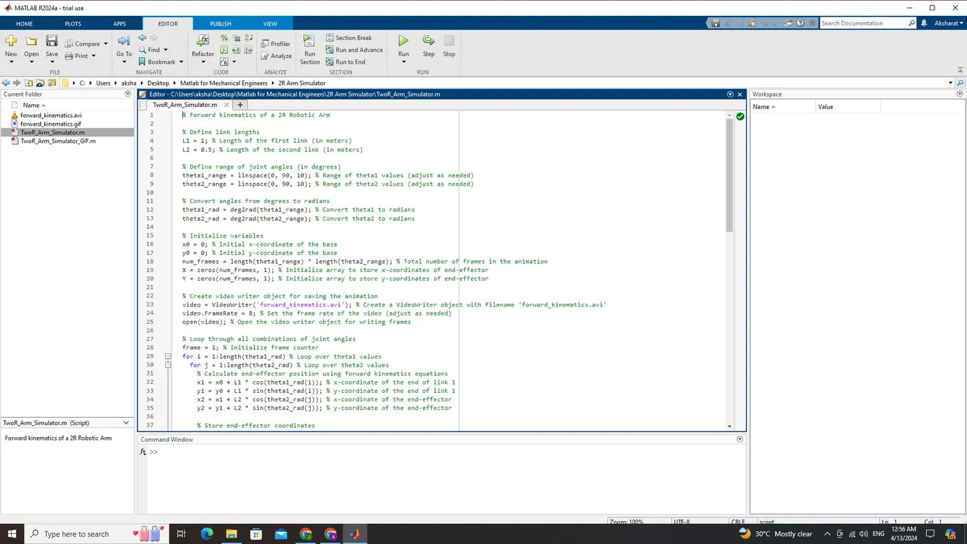
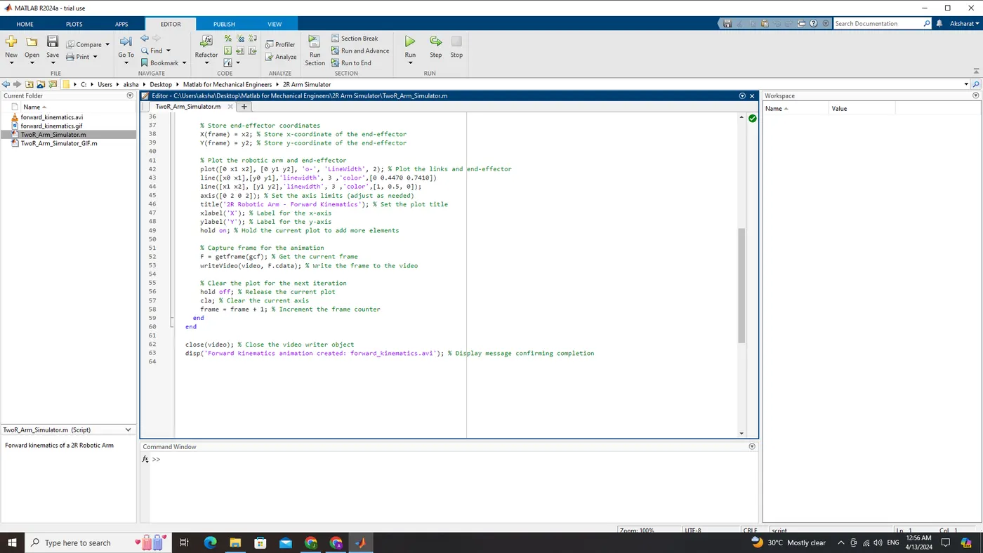
Code for Video

Code for GIF

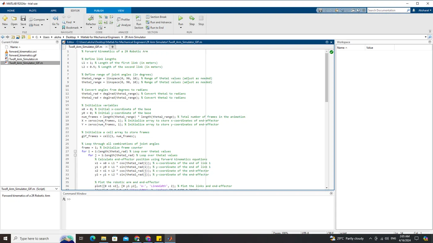
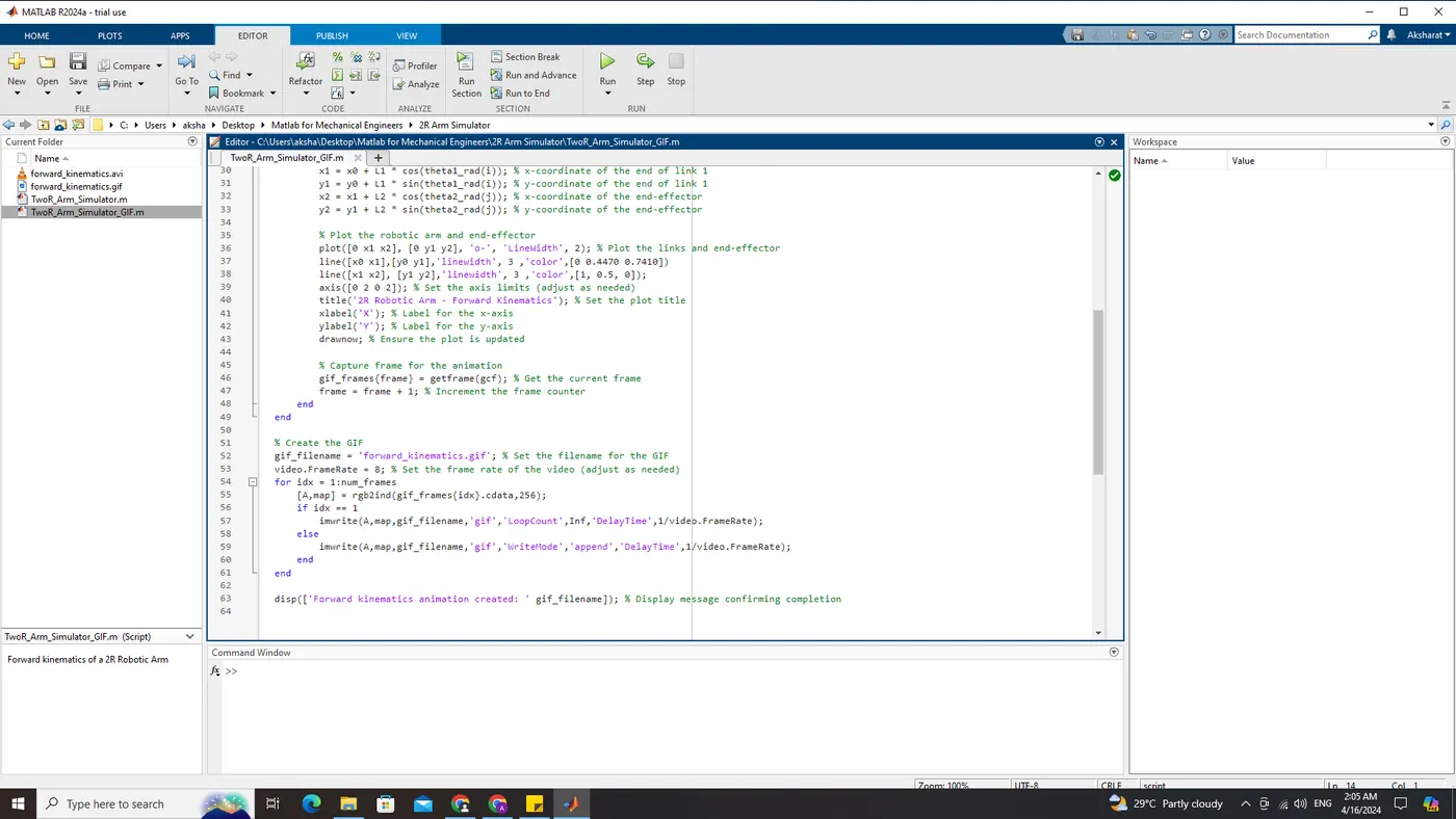
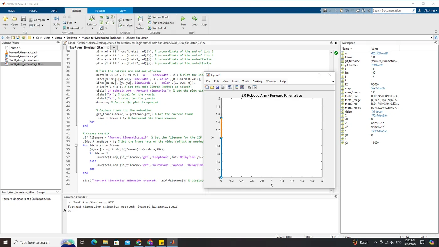
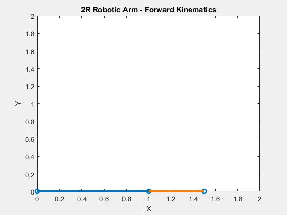
The final output is an animated GIF named forward_kinematics.gif, which shows the movement of the robot manipulator through different configurations as it traverses through the range of joint angles.

Conclusion:

The provided Matlab code model demonstrates the implementation of forward kinematics for a two-link planar robot manipulator. By iteratively calculating the positions of the manipulator's end effector for different combinations of joint angles, the code generates a sequence of plots that depict the movement of the robot manipulator. Overall, this code model offers a practical demonstration of forward kinematics and facilitates a better understanding of robotic arm movements, making it valuable for educational purposes in robotics, engineering, and related fields.

Note:

(I know inside the report it is GIF Image because I couldn't uploaded a video file to the report, but I have two codes for this challenge; 1.) Video Format 2.) GIF Format, I am attaching both the code files along with their output as Video and GIF as a Zip File.)