Week 3.2 - 2R Robotic Arm Challenge

Aim:

The aim of this project is to create an animation of a 2R robotic arm simulation. The 2R robotic arm is a simple yet widely used mechanism in robotics, comprising two revolute joints (R) connected by two rigid links (2). The objective is to visualize the motion of the robotic arm as it changes its working angles.

Problem Statement:

We have a two links of a robotic arm with defined lenght and we need to plot the arm on the graph to find the reachability of arm at different angulations.

also to create set of plots at various positions and to stitch all of them to produce a simulation of 2R robotic arm.

Solution procedure:

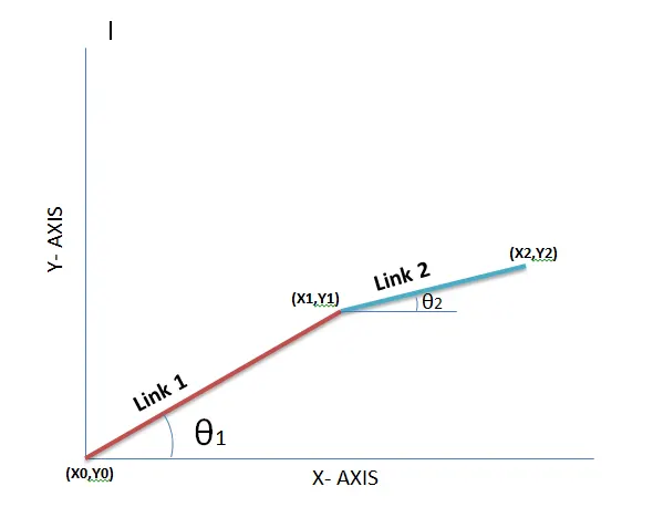
We need to find the cordinate of the all the link end points to draw an arm. in order to find the solution we have two arm arms here i.e: Link 1 and link 2

And we have three cordinate points to be calculated

(X0,Y0) (X1,Y1) and (X2,Y2)

Code:

% Program to animate 2R Robotic arm simulation

% Clearing all the windows
close all
clear all
clc

% Create a folder to store the images
if ~exist('RobotAnimationImages', 'dir')
    mkdir('RobotAnimationImages');
end

% Defining the length of robotic arms in m
l1 = 0.5;
l2 = 0.2;

% Base Coordinates of link 1
x0 = 0;
y0 = 0;

% Counter variable to store the frames
ct = 1;

% Defining the working angles of each arm
theta1 = linspace(0, 90, 10);
theta2 = linspace(0, 90, 10);

% Calcualting the coordinates of each arm for simulation
% We use the nested for loop to generate the working angle for both arms
for i = 1:length(theta1)
    for j = 1:length(theta2)

        % Co ordinates of interconnector of both arms
        x1 = l1 * cosd(theta1(i));
        y1 = l1 * sind(theta1(i));
        
        % Cordinates to define the manipulator
        x2 = x1 + l2 * cosd(theta2(j));
        y2 = y1 + l2 * sind(theta2(j));

        % Plotting the 2R Robotic arm coordinate points
        figure(1);
        plot([x0, x1], [y0, y1], [x1, x2], [y1, y2], 'linewidth', 2);
        axis([-0.2 1 0 1]);
        title('Animation of 2R Robotic arm');
        drawnow;
        
        % Save the image with a unique name based on frame number
        frameImageName = sprintf('RobotAnimationImages/frame_%04d.jpg', ct);
        saveas(gcf, frameImageName);
        
        ct = ct + 1;
    end
end

Output Window:

Explanation:

1. Setting Up the Environment:

   • We start by clearing all open figures, variables, and the command window to ensure a clean workspace for the simulation.

2. Defining Robotic Arm Parameters:

   • We define the lengths of the two links of the 2R robotic arm, l1 and l2, which are 0.5 meters and 0.2 meters, respectively.

3. Initializing Base Coordinates:

   • The base coordinates (x0, y0) are set to (0, 0), representing the starting point of the robotic arm.

4. Defining Working Angles:

   • We create arrays theta1 and theta2 to represent the working angles of each arm.
   • In this code, we chose 10 points equally spaced between 0 and 90 degrees for both angles.

5. Motion Simulation:

   • We use nested for loops to simulate the motion of the 2R robotic arm.
   • The outer loop iterates through each angle in theta1, and the inner loop iterates through each angle in theta2.
   • For each combination of angles, we calculate the (x, y) coordinates of both joints of the robotic arm using trigonometric functions.
   • The cosd function is used to calculate the x-coordinate, and the sind function is used to calculate the y-coordinate.

6. Plotting and Animating the Robotic Arm:

   • For each iteration, we plot the robotic arm by connecting the base (x0, y0) to the first joint (x1, y1) and the first joint to the end effector (x2, y2).
   • The plot function is used to create the lines representing the links of the robotic arm.
   • We set the 'linewidth' to 2 to make the lines more visible.
   • The axis function is used to set the display limits of the plot to maintain a consistent view.
   • The title function is used to set the title of the plot.
   • The drawnow function forces the plot to update before saving the frame as an image.
   • At each iteration, we store the current frame using getframe(gcf) into the variable m. The gcf function returns the handle to the current figure.

7. Saving Animation Frames as Images:

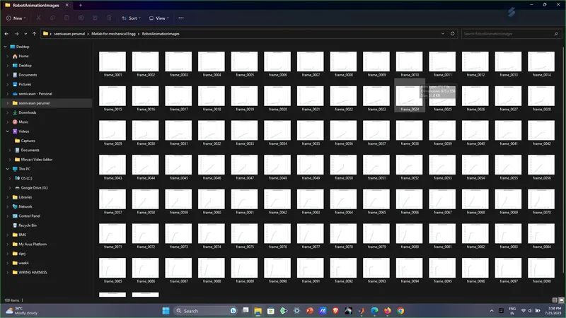
   • After the simulation is complete, we save each frame of the animation as an image in the folder named "RobotAnimationImages".
   • If the folder "RobotAnimationImages" does not exist, the code creates it using the mkdir function.
   • The sprintf function is used to create a filename for each frame, such as "frame_0001.jpg," "frame_0002.jpg," and so on.
   • The imwrite function is used to save the current frame as a JPEG image in the folder with the generated filename.

8. Completion Message:

   • After saving all frames, the code displays a message indicating that the simulation frames have been saved as images in the "RobotAnimationImages" folder.

Challenge Report:

The project report should cover the aim, objective, and detailed explanation of the 2R Robotic Arm Animation code, as mentioned above. It should also discuss the significance of simulating the 2R robotic arm and its applications in real-world scenarios. The report may include sample images from the animation to showcase the motion of the robotic arm at various working angles. Additionally, the report can discuss potential improvements or extensions to the project, such as adding control algorithms to make the robotic arm follow specific trajectories.

Youtube Link:

https://youtu.be/YzdaCUzUkgs