Week 2 Railwheel and Track

Objective

Perform a static structural analysis on the Railwheel and Track setup and

Case 1: Multiply the bearing load by 5 times and compare the results with the load of 100000 N. Compare the Total Deformation, Equivalent stress, and the life under both the loads

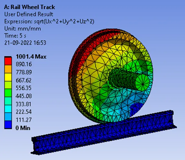
Case 2: Implement a User-defined result and calculate the Total Deformation from this result and check if it is the same as that obtained by the inbuilt result by ANSYS for a load of 100000 N.

CAD Model of the Railwheel and Track is incorporated for Analysis (Front view, Right view & Isometric view)

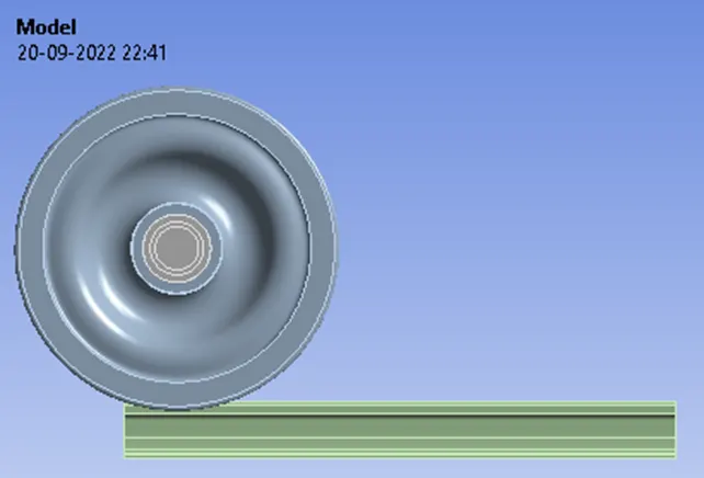
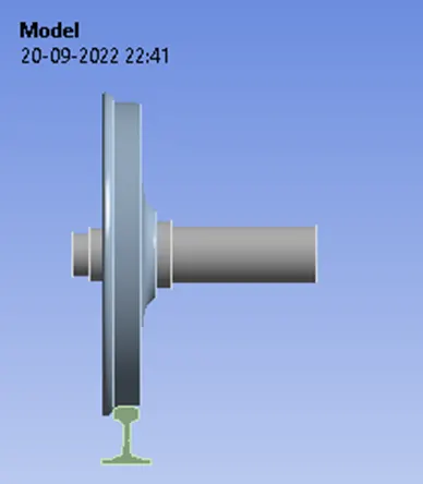
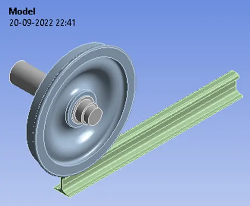
Case 1: Multiply the bearing load by 5 times and compare the results with the load of 100000 N and Compare the Total Deformation, Equivalent stress, and the life under both the loads

Material Used: Structural Steel

Properties of Structural steel:

Density = 7850 kg/m³ , Young’s Modulus E = 210000 MPa, Tensile Yield Strength = 250 MPa, Compressive Yield strength = 250 MPa, Tensile Ultimate Strength = 460 MPa.

Connections

Contact Settings:

Initiating contact settings is crucial for the designer and end-user since the setting of contact surfaces is at the discretion of the designer as to what to ignore and which to consider. Here the Railwheel and Track are in constant contact to undergo dynamic attributes of stresses, strains, and deformations as such the designer have to closely observe and predict the cognitive analytical ability to consider it as crucial for setting the contact region and ignoring other factors for efficient (i.e. Saving Time and Energy) Way of Analysing.

Contacts allowing separation (e.g. frictional contacts) are non-linear contacts. For FE models with non-linear contacts, an iterative process is involved to obtain a solution and therefore non-linear contact analyses are more computationally demanding.

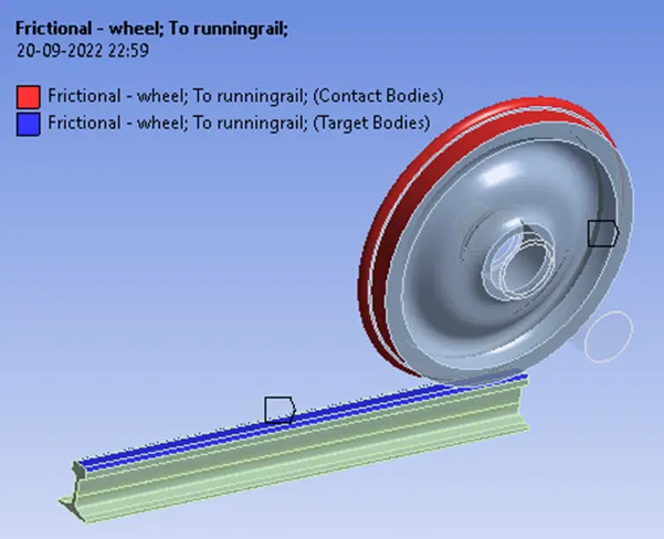
Frictional- Wheel to Running rail

This state is known as “sticking.” The model defines equivalent shear stress (shear stress refers to cases where the deforming force is parallel to a surface) at which sliding on the geometry begins as a fraction of the contact pressure. Once the shear stress is exceeded, the two geometries will slide relative to each other. The coefficient of friction can be any nonnegative value, here we take it as 0.3

shear stress, the force tending to cause deformation of a material by slippage along a plane or planes parallel to the imposed stress.

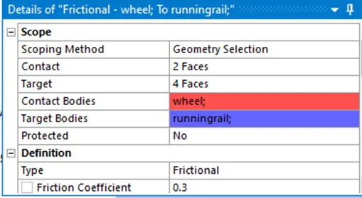
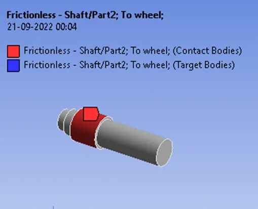
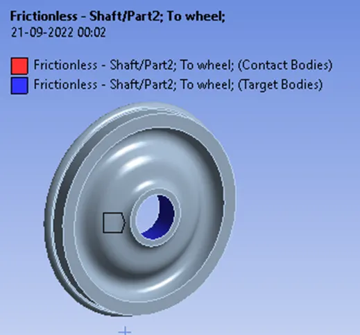
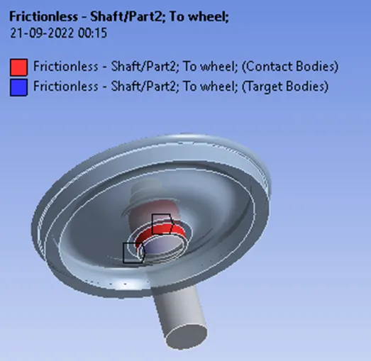
Frictionless – Shaft to Wheel

Frictionless (like easy-flowing, easy-running, smooth-running, laminar, and massless) means no resistance between a surface or substance and something that is moving along or through it.

Joint Settings

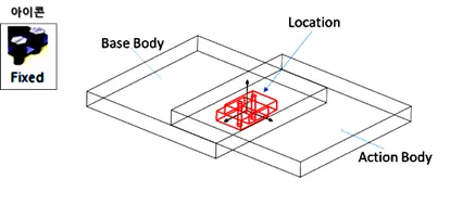
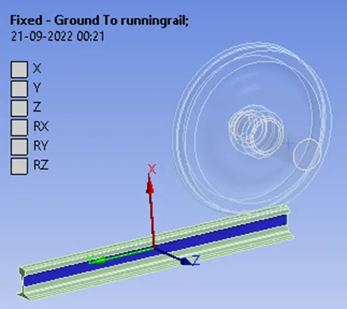
Fixed Joint

The Fixed Joint rigidly connects the two components and does not allow any relative motion between them. It does not add any degrees of freedom.

Translational Joint

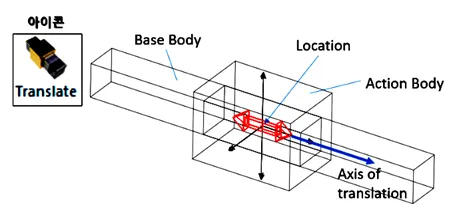
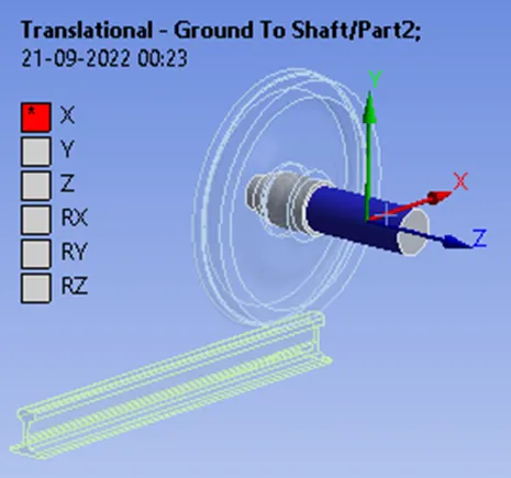
Translational – Ground to Shaft

A translational joint allows the translational movement of two bodies in the direction of a vector defined between the bodies. A translational joint constraints rotational motion in all directions and only allows translational motion in the direction of a specified vector. This means it has only one degree of freedom and constrains the other five degrees of freedom.

Planar Joint

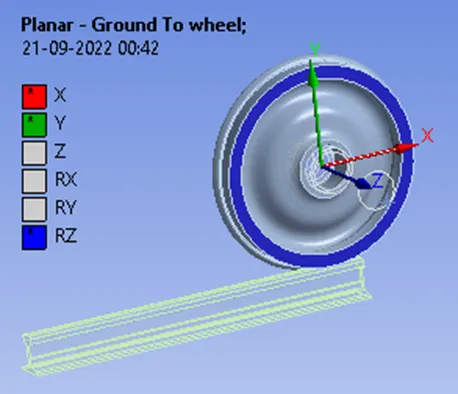
Planar – Ground to wheel

A planar joint only allows the sliding of a body on a plane and its rotational motion about an axis perpendicular to the plane or the Planar Joint has two translational and one rotational degree of freedom between the two components. Both components are free to translate relative to each other in a plane perpendicular to the axis of the joint, and they are also free to rotate about this axis.

Meshing Details

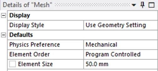
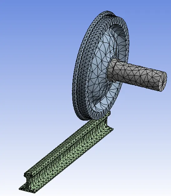
For the meshing part of default solver settings, the ANSYS solver will use the default or recommended mesh value for the model. In this case, since the model looks non-linear with less cross-section and complex geometries take element size as 50mm, hence reducing the element size at the contact surfaces is of much concern for us to achieve precise simulation results for our challenge.

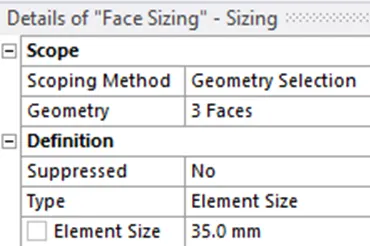
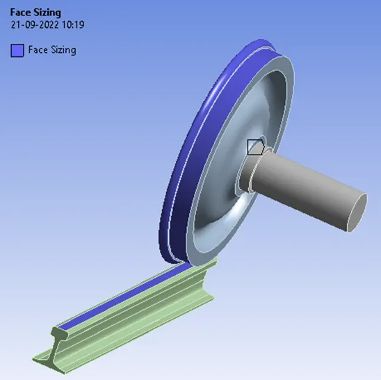
Face sizing is used at the contact surfaces for meshing and taking element size as 35mm. These parameters are used for this particular model and for other cases same is applied.

Mesh Metric:

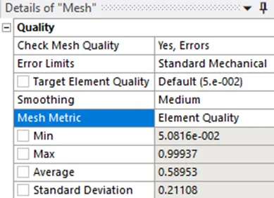
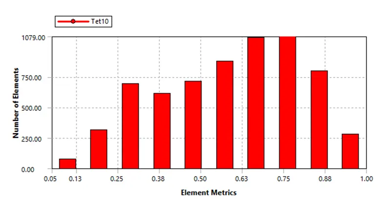
Element Quality

The Element quality option provides a composite quality metric that ranges between 0 and 1 and this metric is based on the ratio of the volume (or area) to the square of the edge length.

So a Value of 1 indicates a perfect cube or square or triangle or hexagon or quad while a Value of 0 indicates that the element has a zero or negative volume

Boundary Conditions

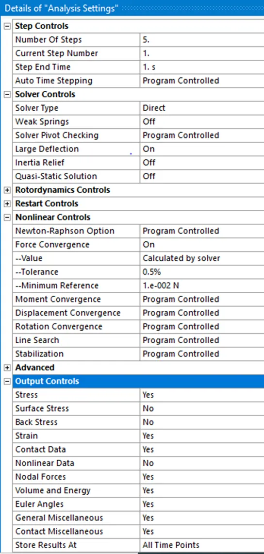
Analysis settings:

The Time Step controls of Analysis settings are crucial for Convergence of Force and Criterion values /curves as this helps the solver converge without any issues.

If we take a smaller time step the solver finds it easy to start with the initial calculation and slowly increases to its maximum time step which helps the solver converges faster without any issues. So always keep this in mind in case you are experiencing any convergence issues try to reduce the time step values and start with a less value so that it helps the solver converge faster

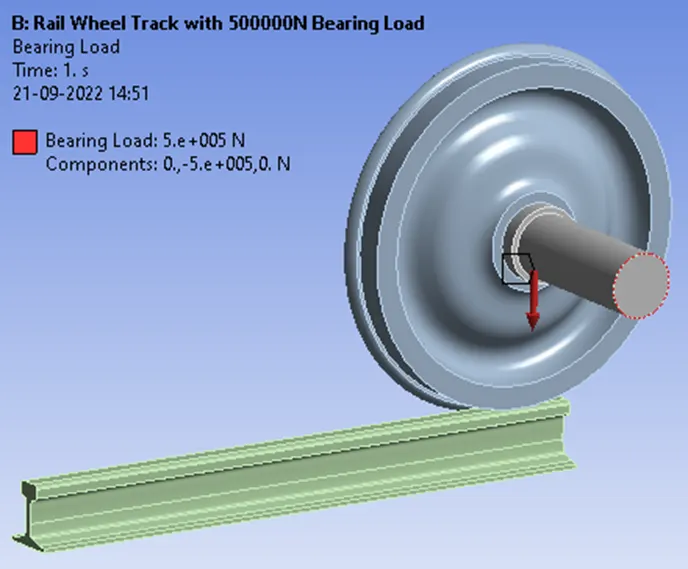
Joint Load Setup

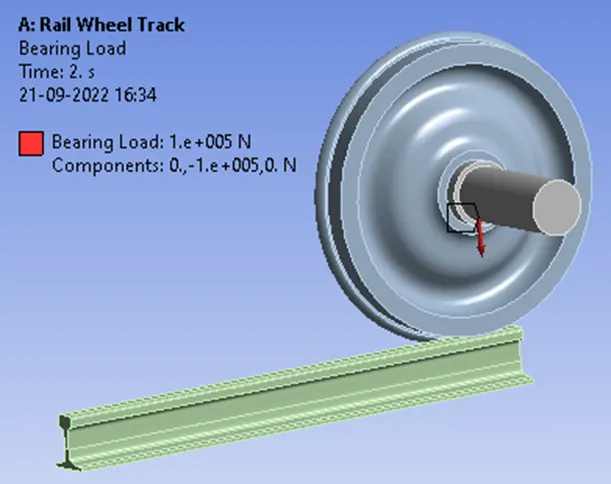
A bearing Load of 500KN is applied on the wheel shaft

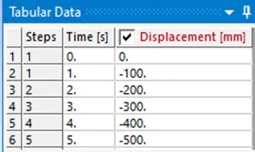
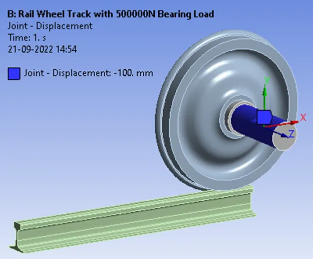
Displacement- Joint

Change in position of the object/rail wheel is analyzed at 100mm for every 5 steps.

Simulation Results

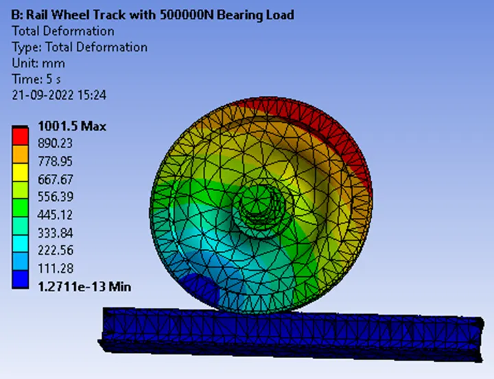
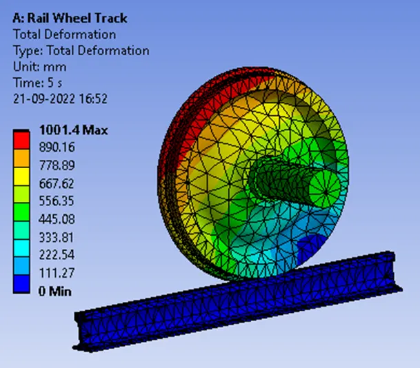
Total Deformation

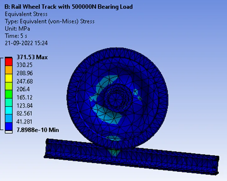
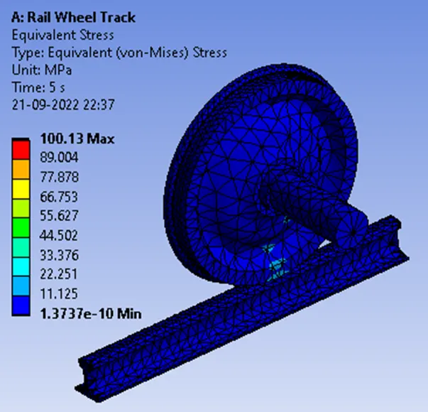
Equivalent Stress

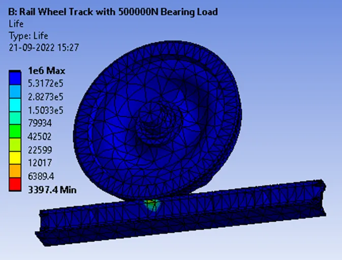
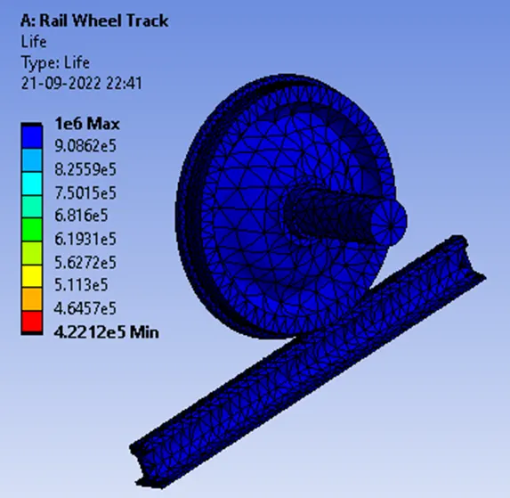
Fatigue Life

User Defined Result

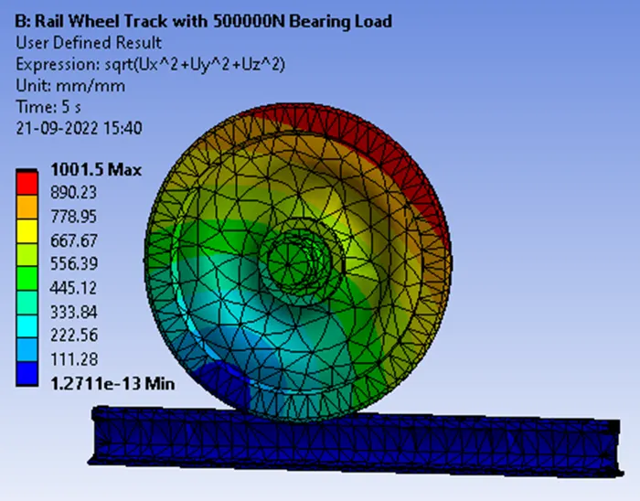
Case 2: Implement a User-defined result and calculate the Total Deformation from this result and check if it is the same as that obtained by the inbuilt result by ANSYS for a load of 100000 N.

Total Deformation at 100 KN

Equivalent stress at 100 KN

Fatigue Life at 100 KN

User Defined results at 100 KN

Concluding Result

Analyzing Cases for	Total Deformation (mm)	Elastic Stress [MPa]	Fatigue Life [MPa]	User Defined Result
100 KN	1001.4 Max	100.13 Max	1e6 Max	1001.4 Max
500 KN	1001.5 Max	371.53 Max	1e6 Max	1001.5 Max

From the above observations of comparative results, we can see a high amount of Stress in the model if we increase the load, as a result of it Stress is going beyond the limit up to 371.53 Mpa thus leading to plastic deformation or permanent deformation can happen.

How?

Here Tensile Yield Strength of Structural Steel is 250 MPa, in the case of 500000 N loads, we got stress as 371.53 MPa which is beyond the limit of the elastic region where plastic deformation or permanent deformation is inevitable. So we should avoid higher loads for safety purposes. Just see the total deformation it is much higher.

User Defined results are the same for both cases.

Fatigue life in 100000 loads and for 500000 loads is the same for both cases.