Week 2 - Flow over a Cylinder.

AIM:

To simulate the flow over a cylinder and explain the phenomenon of karman vortex street.

PART-I

1. Simulate the flow with the steady and unsteady case and calculate the Strouhal Number for Re= 100.

PART-II

1. Calculate the coefficient of drag and lift over a cylinder by setting the Reynolds number to 10,100,1000,10000 & 100000. (Run with steady solver)
2. Discuss the effect of Reynolds number on the coefficient of drag.

INTRODUCTION:

KARMAN VORTEX EFFECT:

In fluid dynamics, a Karman vortex street (or a von Karman vortex street) is a repeating pattern of swirling vortices, caused by a process known as vortex shedding, which is responsible for the unsteady separation of flow of a fluid around blunt bodies.

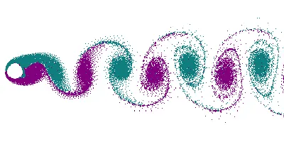
A vortex street will form only at a certain range of flow velocities, specified by a range of Reynolds number (Re), typically above a limiting Re value of about 90. The (global) Reynolds number for a flow is a measure of the ratio of inertial to viscous force in the flow of a fluid around a body or in a channel, and may be defined as a nondimensional parameter of the global speed of the whole fluid flow:

`Re_L = (UL)/ϑ_0`

where:

• U = the free stream flow speed (i.e. the flow speed far from the fluid boundaries U_∞ like the body speed relative to the fluid at rest, or an inviscid flow speed, computed through the Bernoulli equation), which is the original global flow parameter, i.e. the target to be non-dimensionalised.
• L = a characteristic length parameter of the body or channel
• `ϑ_0`= the free stream kinematic viscosity parameter of the fluid, which in turn is the ratio:

`ϑ_0= μ_0/ρ_0`

between:

• `ρ_0`= the reference fluid density.
• `μ_0`= the free stream fluid dynamic viscosity

STROUHAL NUMBER:

This formula will generally hold true for the range 250 < Re_d < 200000:

`St = 0.198 (1-19.7/(Re_d ))`

where:

`St = (fd)/U`

• f= vortex shedding frequency.
• d= diameter of the cylinder
• U= flow velocity.

This dimensionless parameter St is known as the Strouhal number.

REYNOLDS NUMBER:

The Reynolds number (Re) helps predict flow patterns in different fluid flow situations. At low Reynolds numbers, flows tend to be dominated by laminar (sheet-like) flow, while at high Reynolds numbers flows tend to be turbulent. The turbulence results from differences in the fluid's speed and direction, which may sometimes intersect or even move counter to the overall direction of the flow (eddy currents). These eddy currents begin to churn the flow, using up energy in the process, which for liquids increases the chances of cavitation. Reynolds numbers are an important dimensionless quantity in fluid mechanics.

The Reynolds number is the ratio of inertial forces to viscous forces within a fluid which is subjected to relative internal movement due to different fluid velocities.

With respect to laminar and turbulent flow regimes:

• laminar flow occurs at low Reynolds numbers, where viscous forces are dominant, and is characterized by smooth, constant fluid motion;
• turbulent flow occurs at high Reynolds numbers and is dominated by inertial forces, which tend to produce chaotic eddies, vortices and other flow instabilities.

The Reynolds number is defined as,

`Re= (uL)/ϑ= (ρuL)/μ`

where:

• ρ is the density of the fluid (kg/m³)
• u is the flow speed (m/s)
• L is a characteristic linear dimension (m)
• μ is the dynamic viscosity of the fluid (Pa·s or N·s/m² or kg/(m·s))
• ν is the kinematic viscosity of the fluid (m²/s).

DRAG COEFFICIENT:

The drag coefficient (cd) is a dimensionless quantity that is used to determine the drag or resistance of an object in a fluid environment, such as air or water.

The drag coefficient is given as

`c_d= (2F_d)/(ρu^2 A)`

Where:

• A is cross sectional area (m²)
• F_d is drag force (N)
• u is flow velocity (m/s)
• `rho` is the density of the fluid (kg/m³)

LIFT COEFFICIENT:

The drag coefficient (C_L) is a dimensionless quantity that is used to determine the lift of an object in a fluid environment.

The lift coefficient is given as

`c_L= (2F_L)/(ρu^2 A)`

Where:

• A is total area of wings (m²)
• F_L is lift force (N)
• u is flow velocity (m/s)
• `rho` is the density of the fluid (kg/m³)

PROCEDURE:

GEOMETRY CREATION:

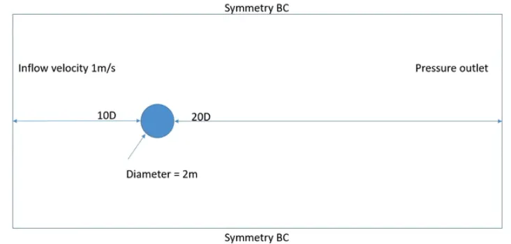
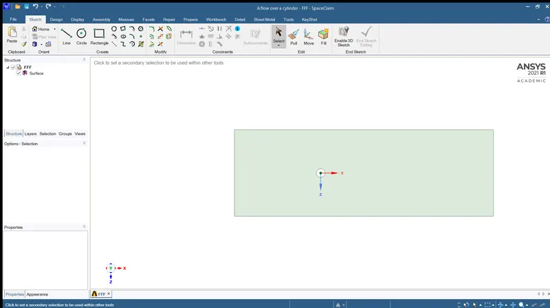
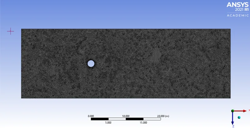
The 2D geometry is created by using the above dimension then the iside cylinder is deleted in order to carry out the simulation.

MESH GENERATION:

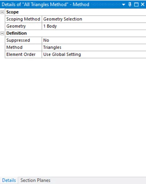
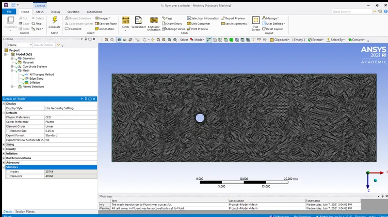
By default Ansys creates the quadrilateral mesh of default size. We need to convert it to triangles.

METHOD:

To change the meshing method. Go to Mesh => insert => method => select face => method (triangles) => generate mesh

SIZING:

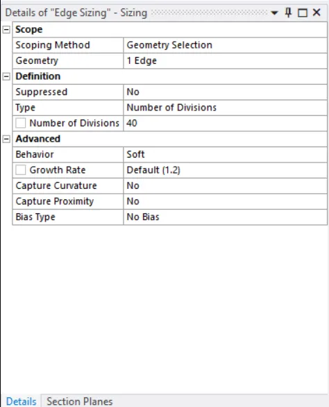
To avoid inaccuracy in solution the sharp corners around the circle are converted into large number of edges.

To do that Go to mesh => insert => sizing => select edge => type (number of divisions) => enter 36 and generate mesh

INFLATION:

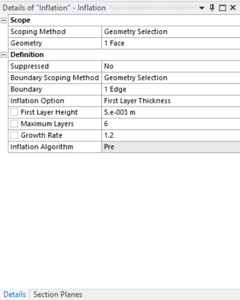
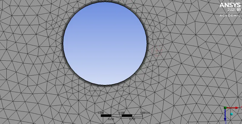
Since the flow around the cylinder is important, the inflation layer is created around the cylinder

To create a inflation layer Go to mesh => insert => inflation => select face => select edge => number of layers => enter number and generate mesh

FINAL MESH:

PART 1:

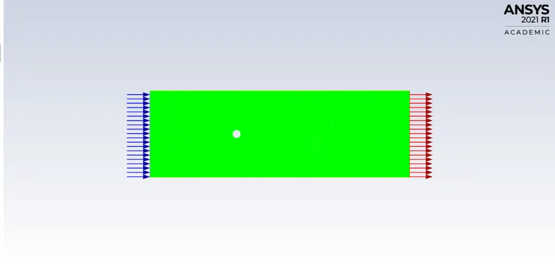
REYNOLDS NUMBER:

For Re = 100:

`Re= (U*ρ*D)/μ`

=>`100 = (U*1*2)/0.02`

U = 1m/s

FLUENT SETUP:

SETUP	STEADY STATE	UNSTEADY STATE
SOLVER TYPE	Pressure based	Pressure based
VELOCITY FORMULATION	Absolute	Absolute
TIME	Steady	Transient
VISCOUS MODEL	Laminar	Laminar
MATERIAL	User defined	User defined
CELL ZONES	Fluid type: user defined Density – 1 kg/m3 Dynamic viscosity – 0.02 kg/ms	Fluid type: user defined Density – 1 kg/m3 Dynamic viscosity – 0.02 kg/ms
BOUNDARIES	Inlet (velocity inlet) Velocity magnitude 1m/s Outlet (pressure outlet) Gauge pressure – 0 pa Symmetry – symmetry Walls – stationary wall Condition - No slip	Inlet (velocity inlet) Velocity magnitude 1m/s Outlet (pressure outlet) Gauge pressure – 0 pa Symmetry – symmetry Walls – stationary wall Condition - No slip

SOLUTION:

• Vertex average of velocity magnitude using surface report at a monitor point at 10m from the center of the cylinder to the right of the cylinder along x-direction.
• Coefficient of drag and coefficient of lift reports are created using force report
• INITIALIZATION: Hybrid for steady state

Standard for unsteady state

• ACTIVITIES: contour plots of pressure and velocity and solution animation are created after initialising the solution.
• RUN CALCULATION:

For steady state – No of iterations= 500

For transient state – Time step = 0.1

No of iterations = 500

RESULTS:

STEADY STATE:

RESIDUAL:

This plot helps in monitoring the change in each and every convergence criterion for every time step and plot those values for every iterations or time step. This plot helps to know when the convergence is achieved.

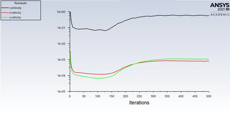
From the above plot we can see that the solution has reached steady state even before 500 iterations.

MONITOR POINT VELOCITY:

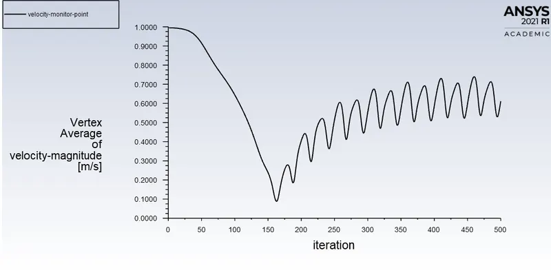
The above plot shows the value of vertex average of velocity magnitude at the monitor point is 0.62 m/s.

CONTOUR:

VELOCITY:

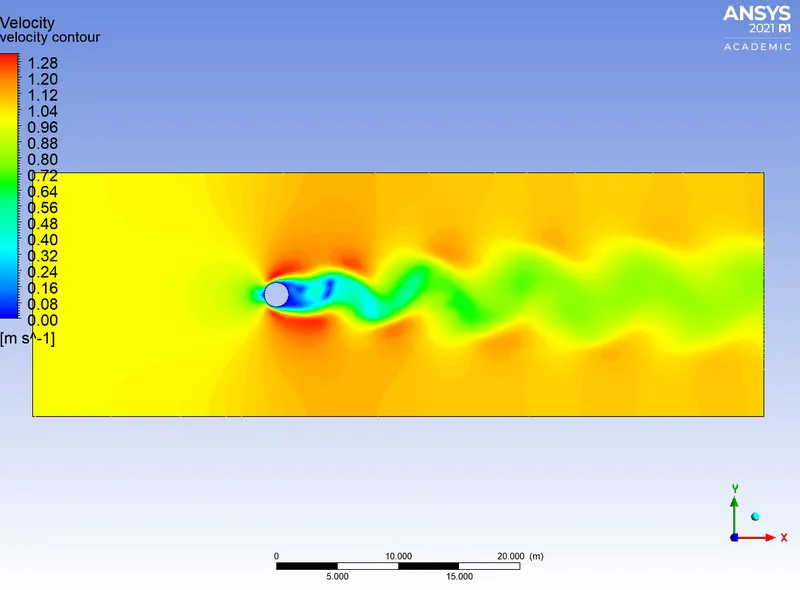
The above contour and animation shows the vortex shedding effect.

PRESSURE:

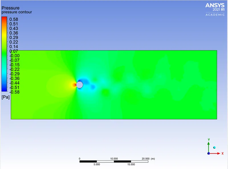
STREAMLINE:

VELOCITY:

The above animation shows the streamline flow for velocity

PRESSURE:

The above animation shows the streamline flow for pressure.

DRAG PLOT:

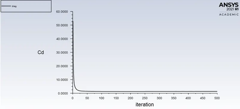
The coefficient of drag plot shows the constant value after certain number of iterations and remains the same after that and the value is 1.367848.

LIFT PLOT:

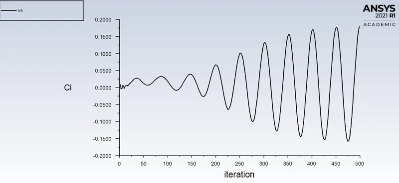
The coefficient of lift plot shows that it starts oscillationg after some times and continues further and the value is 0.17997243.

STROHAUL NUMBER:

The strohaul number cannot be calculated for steady state as we don't calculate the flow with respect to time.

TRANSIENT:

RESIDUAL:

This plot helps in monitoring the change in each and every convergence criterion for every time step and plot those values for every iterations or time step. This plot helps to know when the convergence is achieved.

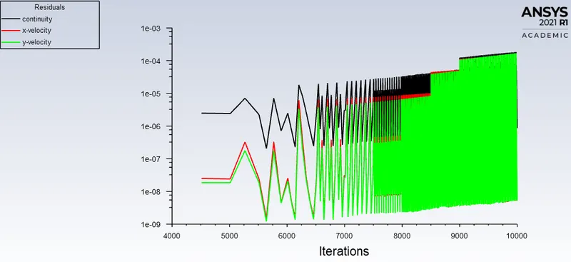
The flow is converged in 3300 iterations.

MONITOR POINT VELOCITY:

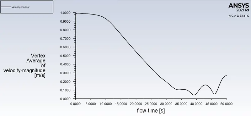
The above plot shows the value of vertex average of velocity magnitude at the monitor point is 0.27 m/s.

CONTOUR:

VELOCITY:

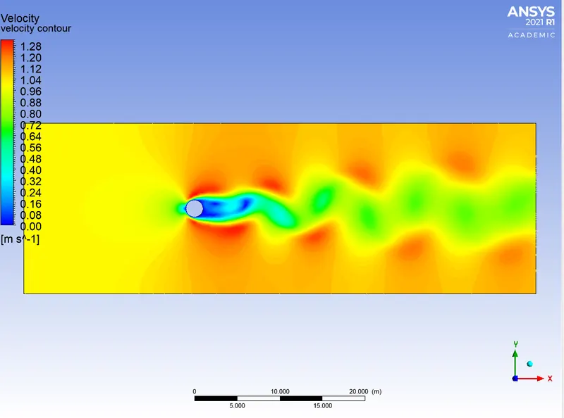
The above contour and animation shows the vortex shedding effect.

PRESSURE:

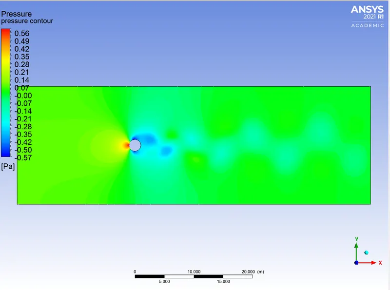
DRAG PLOT:

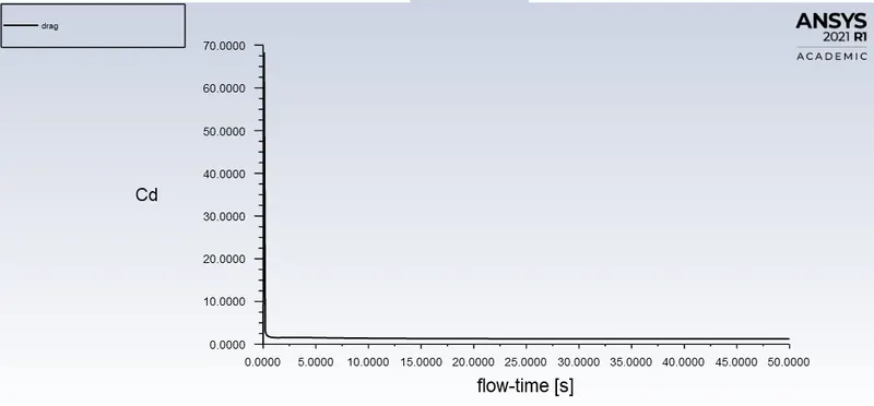
The coefficient of drag plot shows the constant value after certain number of iterations and remains the same after that and the value is 1.2657366.

LIFT PLOT:

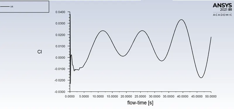
The coefficient of lift plot shows that it starts oscillationg after some times and continues further and the value is 0.018048622.

STROHAUL NUMBER:

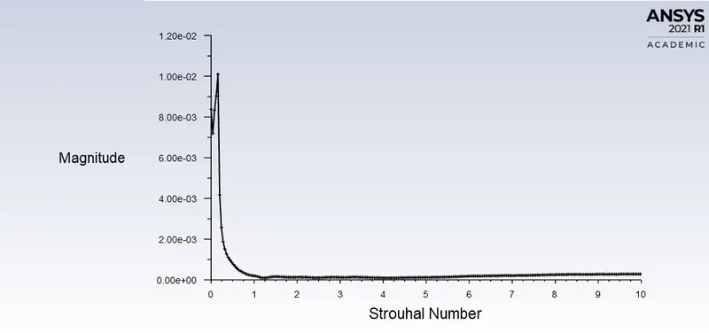
Strohaul number = 0.01.

SUMMARY:

CASES	REYNOLDS NUMBER	INLET VELOCITY	Cd	Ci	MONITOR VELOCITY
STEADY STATE	100	1m/s	1.367848	0.17997243	0.62m/s
TRANSIENT STATE	100	1m/s	1.2657366	0.018048622	0.27m/s

From the above cases we can say that in transient case the velocity starts oscillating for the monitoring point after certain iterations and the velocity at monitoring point is greater in case of steady state case as compared to transient case.

PART 2:

CASE 1:

SIMULATION OF FLOW FOR THE STEADY STATE FOR Re = 10

Velocity calculation for Reynolds number 10,

For Re = 10:

`Re= (U*ρ*D)/μ =>10 = (U*1*2)/0.02`

U = 0.1m/s

RESULTS:

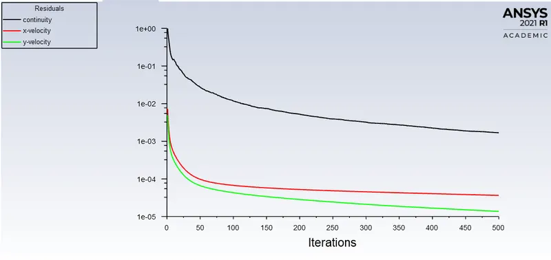
RESIDUAL:

This plot helps in monitoring the change in each and every convergence criterion for every time step and plot those values for every iterations or time step. This plot helps to know when the convergence is achieved.

MONITOR POINT VELOCITY:

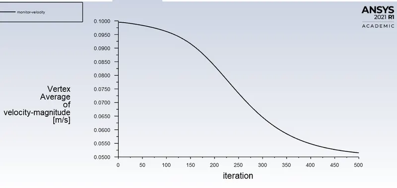
From this plot we can see that for re = 10 there is no oscillations in velocity.

VELOCITY CONTOUR:

From the animation we can see that there is no vortex shedding formation when reynolds number 10.

DRAG PLOT:

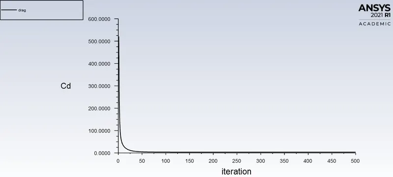
The value of cd is 3.3314425.

LIFT PLOT:

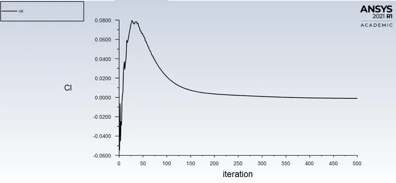
The value of cl is -0.00085925251.

CASE 2:

SIMULATION OF FLOW FOR THE STEADY STATE FOR Re = 100

Velocity calculation for Reynolds number 100,

For Re = 100:

`Re= (U*ρ*D)/μ =>100 = (U*1*2)/0.02`

U = 1m/s

RESULTS:

RESIDUAL:

This plot helps in monitoring the change in each and every convergence criterion for every time step and plot those values for every iterations or time step. This plot helps to know when the convergence is achieved.

MONITOR POINT VELOCITY:

This above plot shows the vertex average of velocity magnitude at the monitor point is 0.61154234

VELOCITY CONTOUR:

The above animation shows the vortex shedding formation.

DRAG PLOT:

the value of cd is 1.367848.

LIFT PLOT:

the value of cl is 0.17997243.

CASE 3:

SIMULATION OF FLOW FOR THE STEADY STATE FOR Re = 1000

Velocity calculation for Reynolds number 1000,

For Re = 1000:

`Re= (U*ρ*D)/μ =>1000 = (U*1*2)/0.02`

U = 10m/s

RESULTS:

RESIDUAL:

This plot helps in monitoring the change in each and every convergence criterion for every time step and plot those values for every iterations or time step. This plot helps to know when the convergence is achieved.

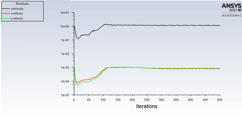
MONITOR POINT VELOCITY:

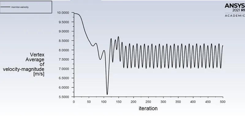
The above plot shows the vertex average of velocity magnitude at the monitor point is 8.2080564

VELOCITY CONTOUR:

The above animation shows the vortex shedding formation.

DRAG PLOT:

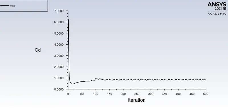
The value of cd is 0.86912317.

LIFT PLOT:

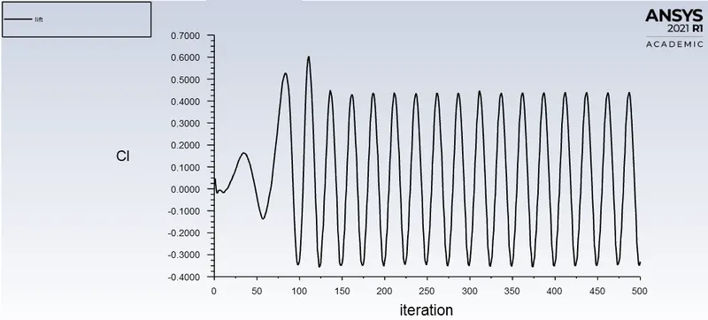
The value of cl is -0.331299.

CASE 4:

SIMULATION OF FLOW FOR THE STEADY STATE FOR Re = 10000

Velocity calculation for Reynolds number 10000,

For Re = 10000:

`Re= (U*ρ*D)/μ =>10000 = (U*1*2)/0.02`

U = 100m/s

RESULTS:

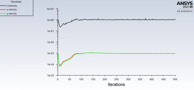
RESIDUAL:

This plot helps in monitoring the change in each and every convergence criterion for every time step and plot those values for every iterations or time step. This plot helps to know when the convergence is achieved.

MONITOR POINT VELOCITY:

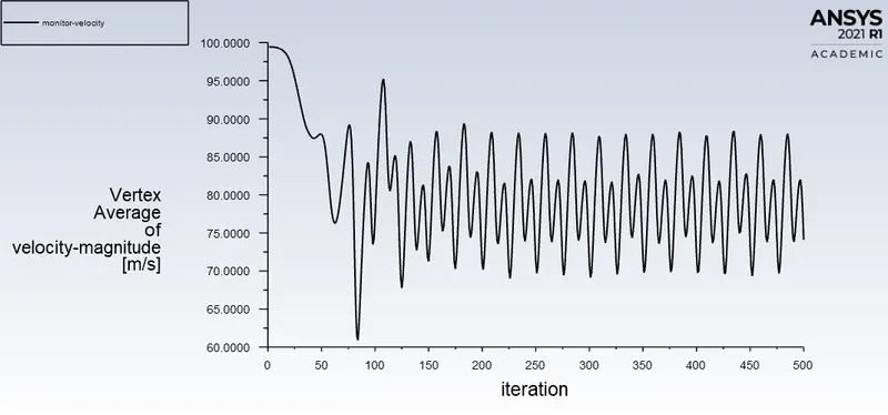
The above plot shows the vertex average of velocity magnitude at the monitor point is 74.108414

VELOCITY CONTOUR:

The above animation shows the vortex shedding fomation.

DRAG PLOT:

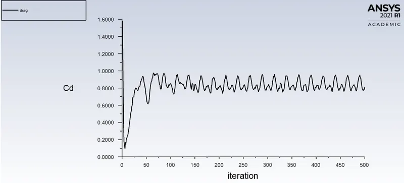
The value of cd is 0.81047329.

LIFT PLOT:

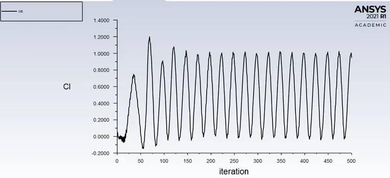
The value of cl is 0.9461438.

CASE 5:

SIMULATION OF FLOW FOR THE STEADY STATE FOR Re = 100000

Velocity calculation for Reynolds number 100000,

For Re = 100000:

`Re= (U*ρ*D)/μ =>100000 = (U*1*2)/0.02`

U = 1000m/s

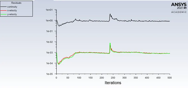
RESULTS:

RESIDUAL:

This plot helps in monitoring the change in each and every convergence criterion for every time step and plot those values for every iterations or time step. This plot helps to know when the convergence is achieved.

MONITOR POINT VELOCITY:

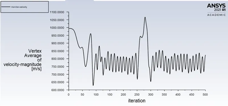
The above plot shows the vertex average of velocity magnitude at the monitor point is 824.28937 m/s

VELOCITY CONTOUR:

The above animation shows the vortex shedding formation.

DRAG PLOT:

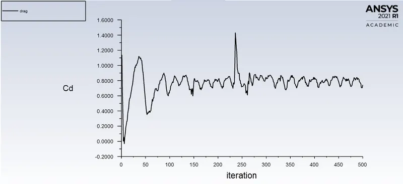
The value of cd is 0.74380507

LIFT PLOT:

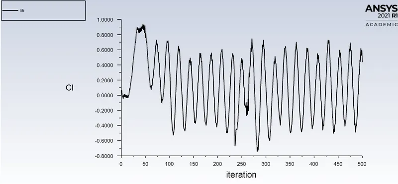
The value of cl is 0.43716453

SUMMARY:

CASE	REYNOLDS NUMBER	Cd	Cl
1	10	3.3314425	-0.00085925251
2	100	1.367848	0.17997243
3	1000	0.86912317	-0.331299
4	10000	0.81047329	0.9461438
5	100000	0.74380507	0.43716453

From the above plot we can say that the value of lift coefficient keeps on increasing as we keep increasing the velocity and Reynolds number. The drag coefficient is maximum for lowest Reynolds number and goes on decreasing.

CONCLUSION:

• When fluid flows over the cylinder, wake region is formed next to cylinder due to decrease in pressure and recirculation of flow occurs and hence flow separation occurs.
• As flow over cylinder is being transient we are unable to observe flow separation at low Reynolds number
• As the Reynolds number increases the coefficient of drag decreases.
• Strauhal number for unsteady state with Reynolds number 100 is 0.01.

REFERENCE MATERIAL:

Numerical simulation of laminar flow past a circular cylinder - ScienceDirect

https://www.grc.nasa.gov/WWW/wind/valid/lamcyl/Study1_files/Study1.html

Paper Title (use style: paper title) (flowvisioncfd.com)