Week 2 - Flow over a Cylinder.
Objective :
1) Explain phenomenon of Karman-Vortex street
2) Set up a simulation for flow over a cylinder
a)Simulate the flow with the steady and unsteady case and calculate the Strouhal Number for Re= 100.
b)Calculate the coefficient of drag and lift over a cylinder by setting the Reynolds number to 10,100,1000,10000 & 100000. (Run with steady solver)
3)Discuss the effect of Reynolds number on the coefficient of drag. [ Results should be validated with any standard literature and error should be within 5 %]
Introduction :
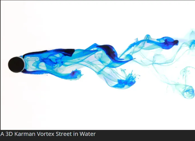
A Karman Vortex street is a repeating pattern of swirling vortices, caused by a process known as vortex shedding, which is responsible for the unsteady seperation of flow of a fluid around blunt bodies. This phenomen is observed for cylinders in fluids with Reynolds Number ranging from 100 to `10^5` . This causes a force on the cylinder perpendicular to the flow that reverses direction each time a vortex is shed. Such vortex shedding is why flags flap and taut wires hum in the wind. If the frequency of vortex shedding is close to the natural frequency of some mode of vibration of the cylinder body, then an appreciable lateral vibration culminates.An understanding of the transitional flow processes will help in practical problems either by improving procedures for predicting positions or for determining methods of advancing or retarding the transition position.
Simulation Set up :
1) Geometry :
A rectangular section was created with a circle whose center is at origin . 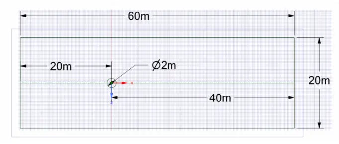
Pull tool was used to extract the rectangular surface with a circular hole .
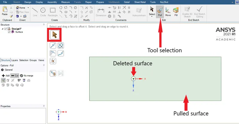
Thus the required geomtery was created . The space claim was closed and mesh module was updated before opening .
Meshing :
Boundary conditions were given to the model .
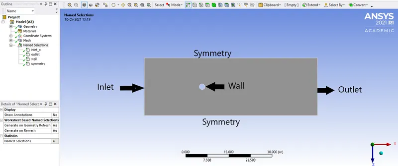
Mesh was generated with element length as 0.25m
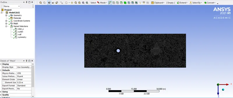
Edge sizing and inflation tools were used to divide the circle into a number of parts and create quad elements near the circumference of the wall so the results can be captured better .
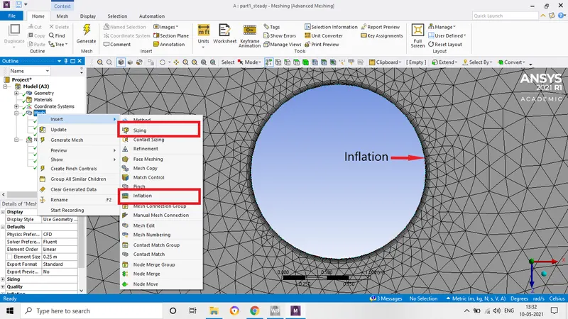
Thus meshing was completed and mesh module was closed . The set up module was updated and opened .
Set up :
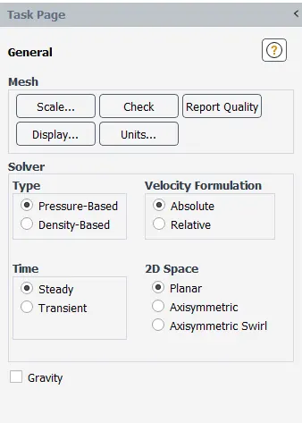
The general solver setting was made as pressure based , steady state with absolute velocity formulation.
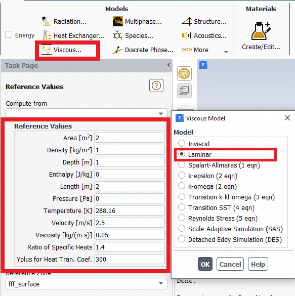
Model type was set to viscous laminar and Reference values were set as follows .
Material was manually created with all properties same as that of air except density and viscosity.
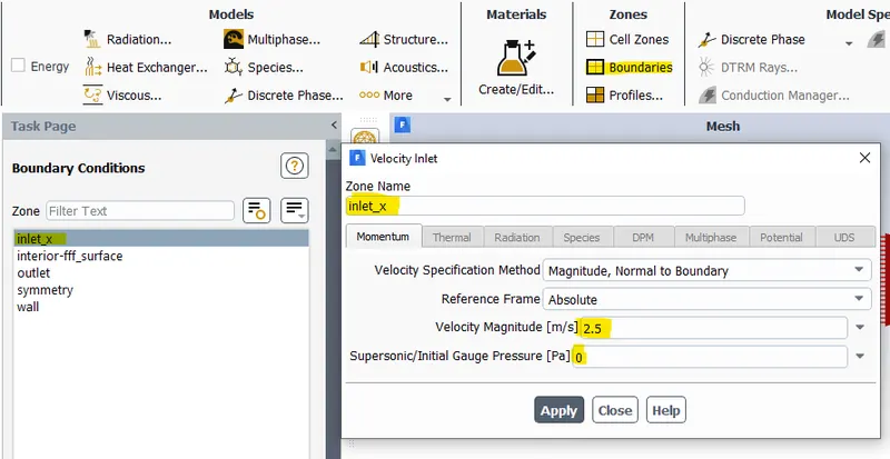
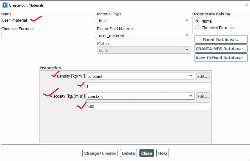 Values for boundary conditions were entered . In this case Re=100 , hence Velocity=2.5m/s .
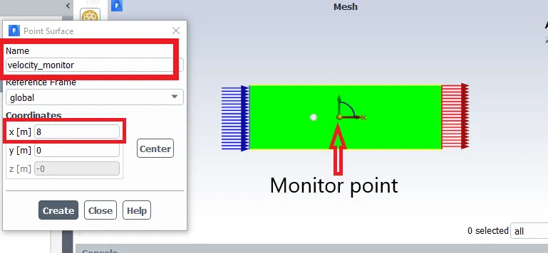
A monitor point was created 8m from centre of circle in the positive x direction .
The following residuals were created
a) Co-efficient of lift at wall
b) Co-efficient of drag at wall
c) Vertex-average velocity at the monitor point.
Contours for velocity and pressure were created .
Thus we have set up the case as per given requirements .
Results :
1)Part 1
Case 1 :
Solver type for time : Steady
Re=100
Velocity : 2.5m/s
Density : 1kg/m^3
Viscosity : .05 kg/(m.s)
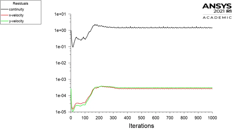
Scaled Residual plot
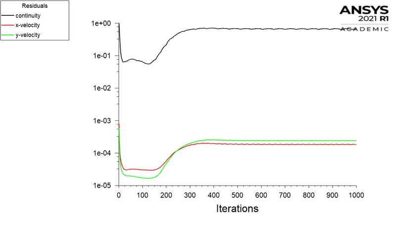
Velocity plot
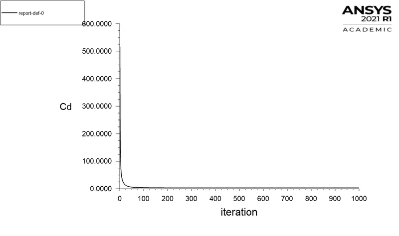
Co-efficient of drag
Co-efficient of Lift
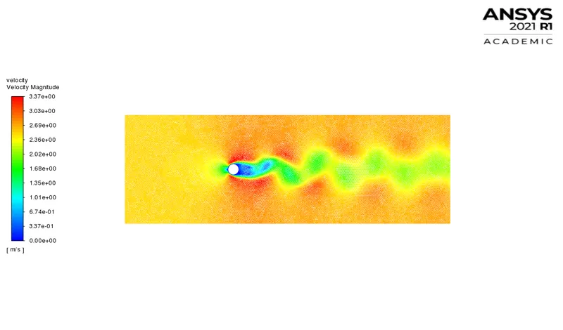
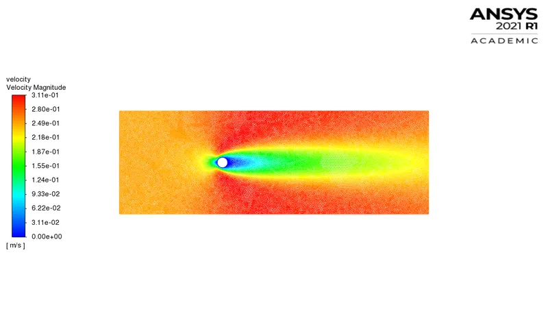
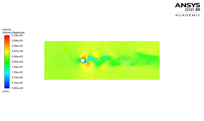
Velocity contour
Case 2 :
Solver type for time : Unsteady
Re=100
Velocity : 2.5m/s
Density : 1kg/m^3
Viscosity : .05 kg/(m.s)
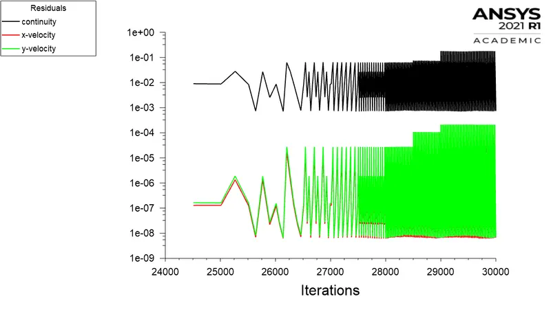
Scaled Residual plot
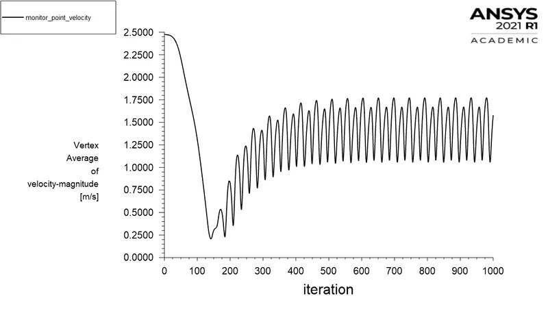
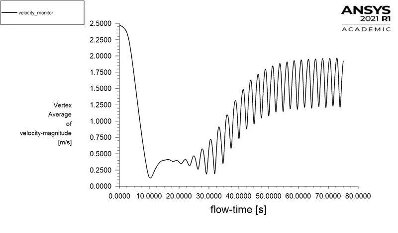
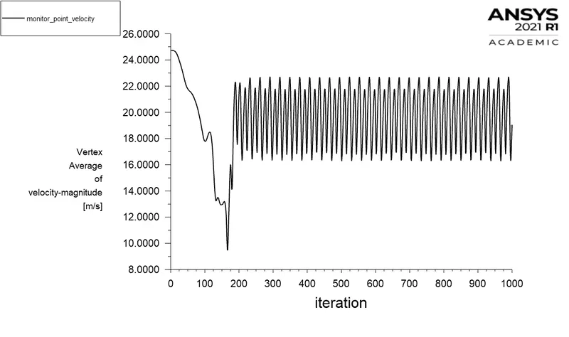
Monitor point Velocity plot
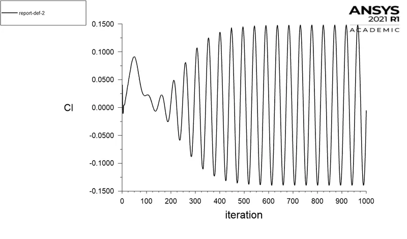
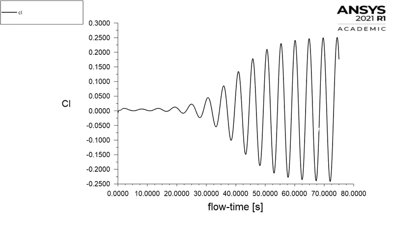
Co-efficient of lift
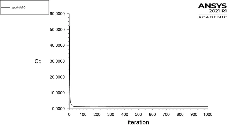
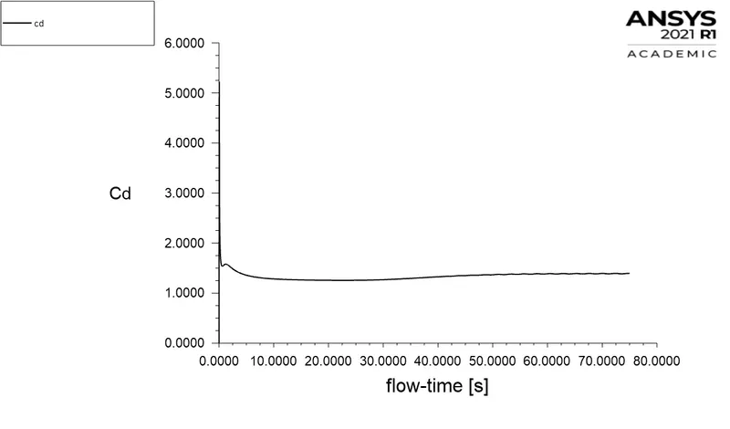
Co-efficient of drag
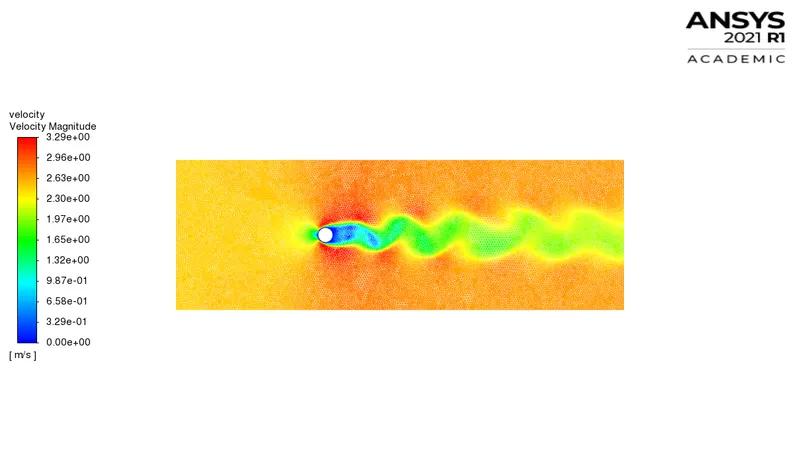
Velocity contour
Part 2 :
Case 1:
Solver type for time : Steady
Re=10
Velocity : 0.25m/s
Density : 1kg/m^3
Viscosity : .05 kg/(m.s)
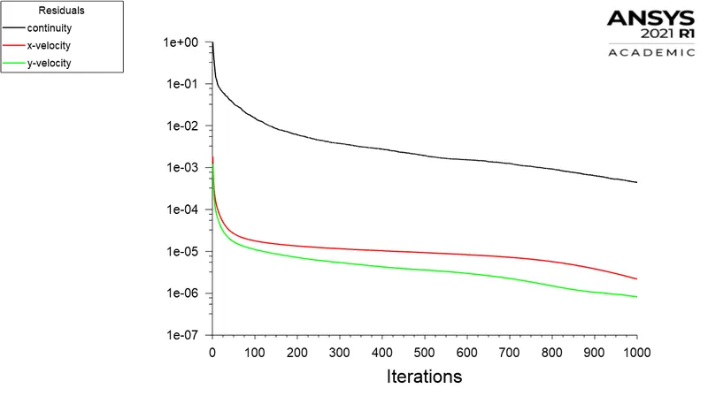
Scaled Residuals
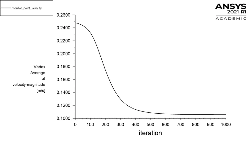
Monitor Point Velocity plot
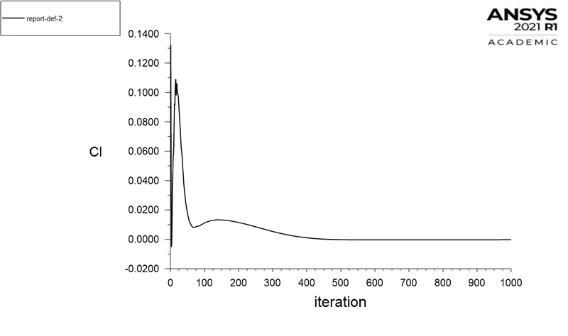
Co-efficient of Lift
Co-efficient of Drag
Velocity Contour
Case 2:
Solver type for time : Steady
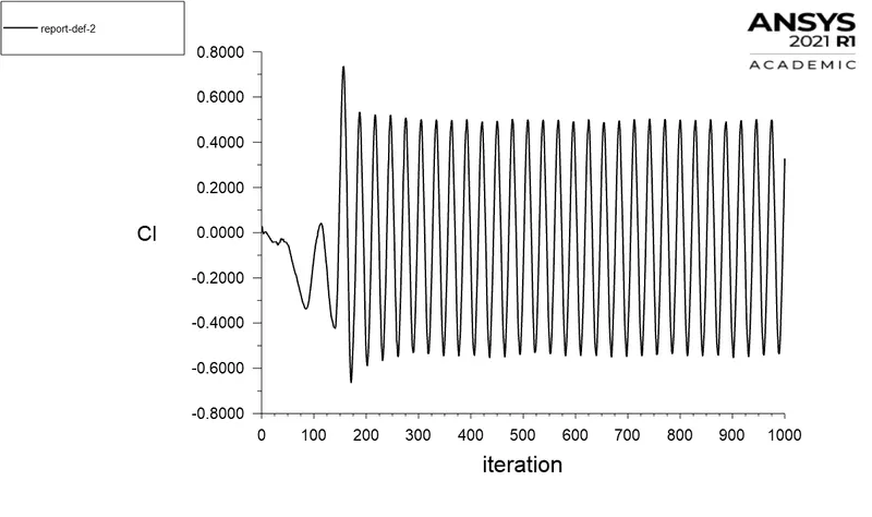
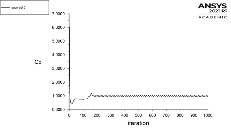
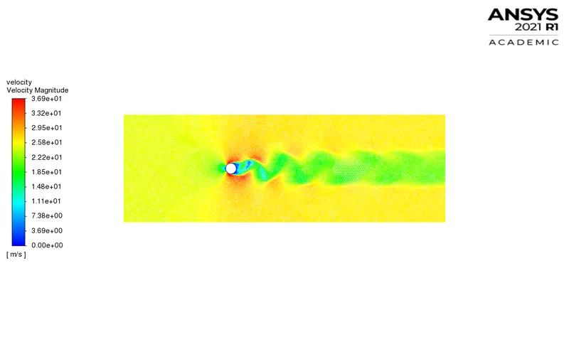
Re=1000
Velocity : 25m/s
Density : 1kg/m^3
Viscosity : .05 kg/(m.s)
Scaled Residuals
Monitor Point Velocity plot
Co-efficient of Lift
Co-efficient of Drag
Velocity Contour
Case 3:
Solver type for time : Steady
Re=10000
Velocity : 250 m/s
Density : 1kg/m^3
Viscosity : .05 kg/(m.s)
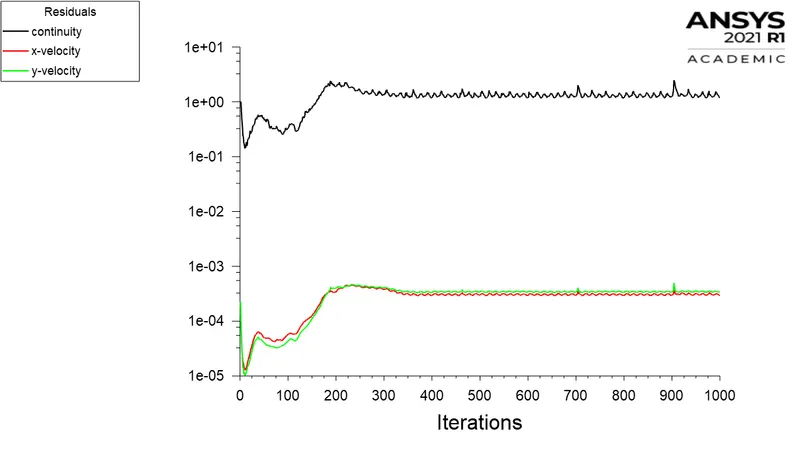
Scaled Residuals
Monitor Point Velocity plot
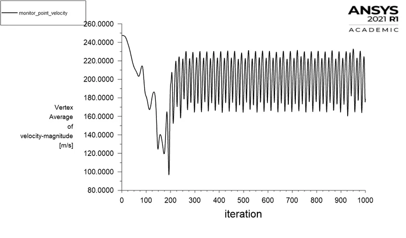
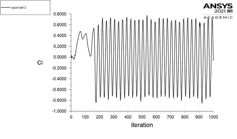
Co-efficient of Lift
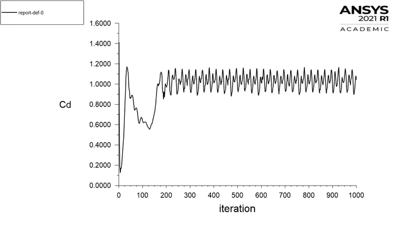
Co-efficient of Drag
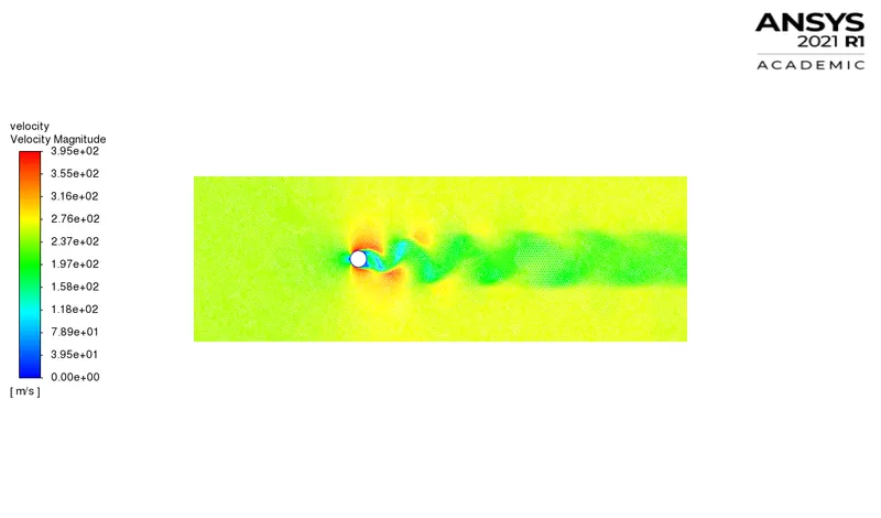
Velocity Contour
Case 4:
Solver type for time : Steady
Re=100000
Velocity : 2500 m/s
Density : 1kg/m^3
Viscosity : .05 kg/(m.s)
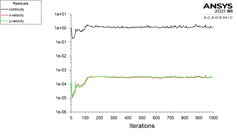
Scaled Residuals
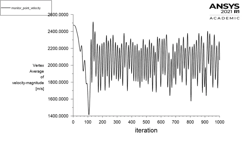
Monitor Point Velocity plot
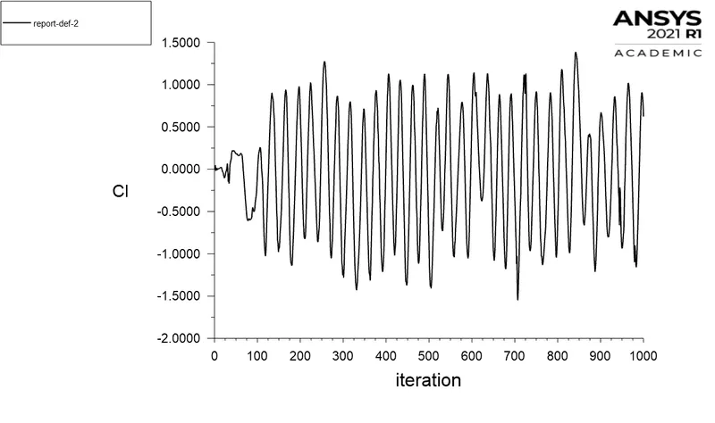
Co-efficient of Lift
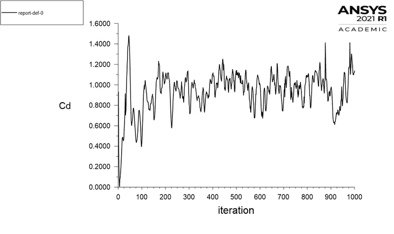
Co-efficient of Drag
Velocity Contour
Inference :
1) Simulation was run with steady and unsteady solver , Re=100 and strouhall number was calculated for unsteady case.
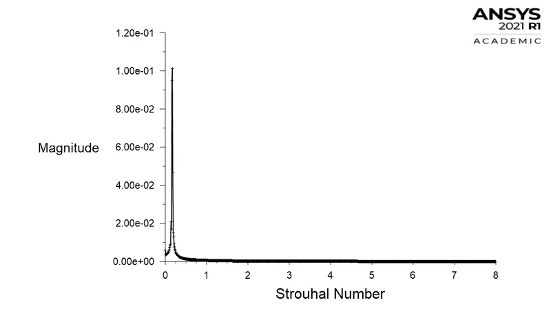
Value of stouhall number obtained = 0.171
2) Simulation was run with various Reynolds number , Results are tabulated below .
| Sl No | Reynolds Number | Co-efficient of Lift | Co-efficient of Drag |
| 1 | 10 | -0.000241 | 3.333 |
| 2 | 100 (Steady) | -0.005098 | 1.349 |
| 3 | 100 (Unsteady) | 0.175896 | 1.394 |
| 4 | 1000 | 0.3277 | 0.923 |
| 5 | 10000 | -0.0613 | 1.042 |
| 6 | 100000 | 0.6224 | 1.137 |
Vortex shedding is not observed for very low Re values .
For Re=100 ,
Theoretical value of Cd = 1.335
Numerical value of Cd =1.349
Hence we have validated our solution . Percentage Error is < 5% .
We can observe that Drag co-efficient reduces as Reynolds number increases till Re=4000. Then the Drag co-efficient seems to increase slightly .
Reference Research Paper:- https://www.sciencedirect.com/science/article/pii/S0307904X08000243