Week 2 - Flow over a Cylinder.
OBJECTIVE ;
To Simulate the flow over a cylinder and explain the phenomenon of Korman vortex . In this simulation there are two cases solved as follows
CASE 1
- Simulating the flow in a steady and Unsteady state when Reynolds number = 100 and deriving Strouhal number from the simulation
CASE 2
- Simulating the flow in a steady state for Reynolds number 10,100,1000,10000, and 100000. Calculating Drag coefficient and Lift coefficient for this study.
PROCEDURE:
Simulating the flow for the above mentioned cases are done in a step wise progress in the ANSYS FLUENT. These steps are regulated on the problem in a demand wise for how the simulation responds ,i.e study involving parametrical changes in the physical condition of the simulaion.
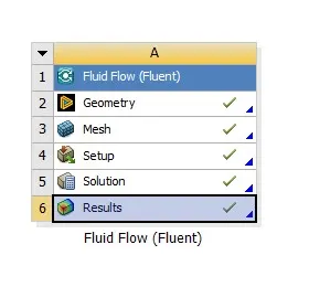
ANSYS FLUENT works on the flow starting from the geometry creating meshing then solving the meshed geometry to imprintinhg the results on post processing. The results simulated from solving the cases give us a detailed analogy for the problem.
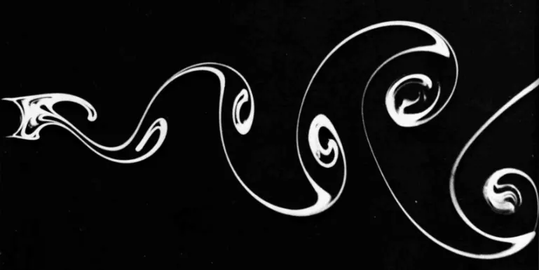
KARMAN VORTEX STREET
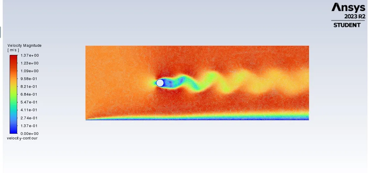
The phenomena of producing a swirling vortices when a flow hits a material characterised with a frequency of shedding is known as Karman vortex shedding. These are caused due to flow separation which then leads to a pressure difference on the flow approach which results invortex shedding.
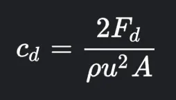
DRAG COEFFICIENT :
Drag coefficient is used to quantify the drag resistance in a flow. It is a Dimensionless quantity and the formula goes by
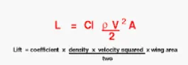
LIFT COEFFIENT :
Lift coeeficient is Dimensionless quantity that is used to quantify the lift generated in a object when it approaches a flow due to the fluid density and the fluid velocity around the material
ANSYS FLUENT WORKFLOW
SETTING UP GEOMETRY
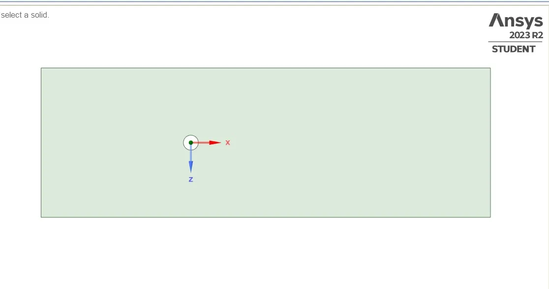
The cylinder centralised on the origin acts as the material interacts with the flow flowing from right to left.
MESHING
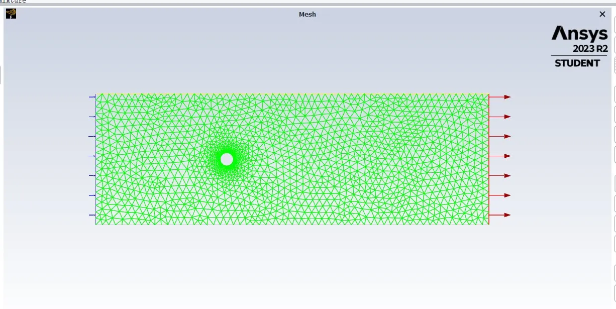
Boundary conditions are defined and meshed on the geometry for further solving and processing.
- Mesh unit dimension is set to 0.5 metre and 6 inflation layers are added for extracting the flow condition without any disturbances or diversion at the boundary of the material wall
SETUP
Solving for the part 1
- DEFINTION :
Simulating steady and unsteady states on the simulation for a flow over a cylinder when Reynolds number = 100 and calculating the strouhal number for the unsteady state.
SETUP AND SIMULATION
STEADY STATE ANALYSIS
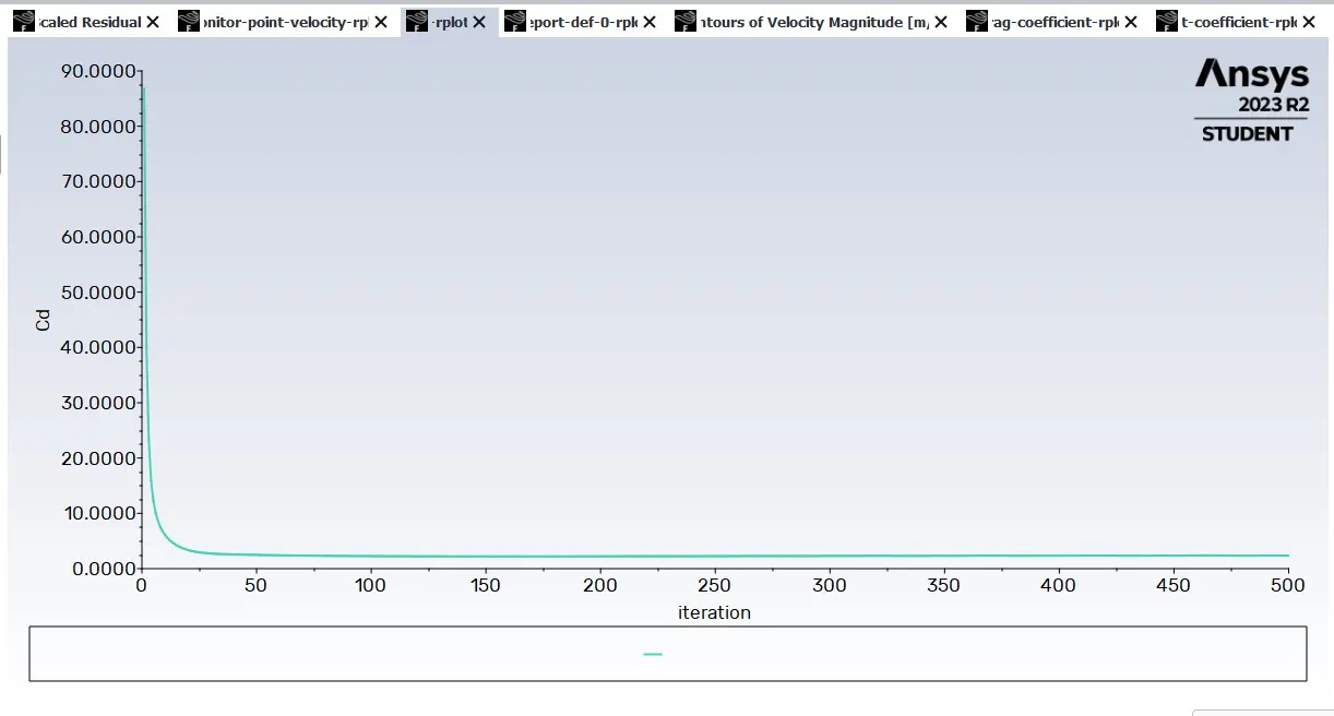
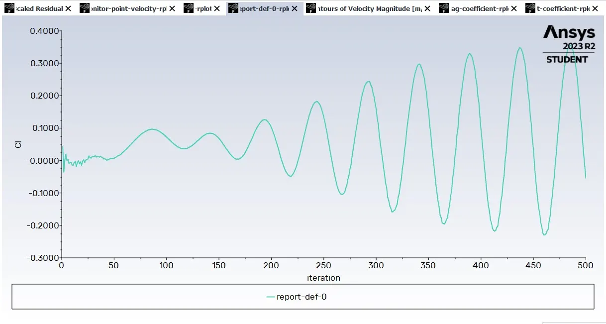
For Reynolds number Re = 100
The simulation goes like
SCALED RESIDUAL
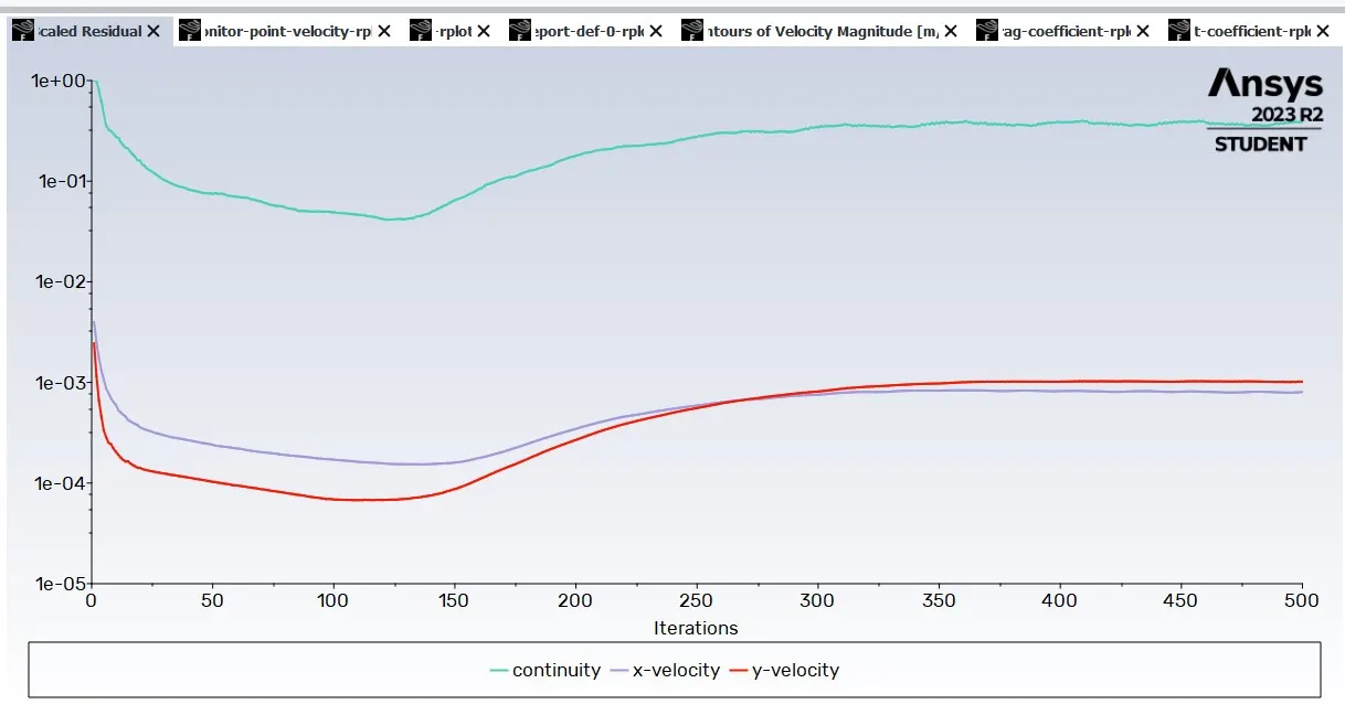
MONITOR POINT VELOCITY
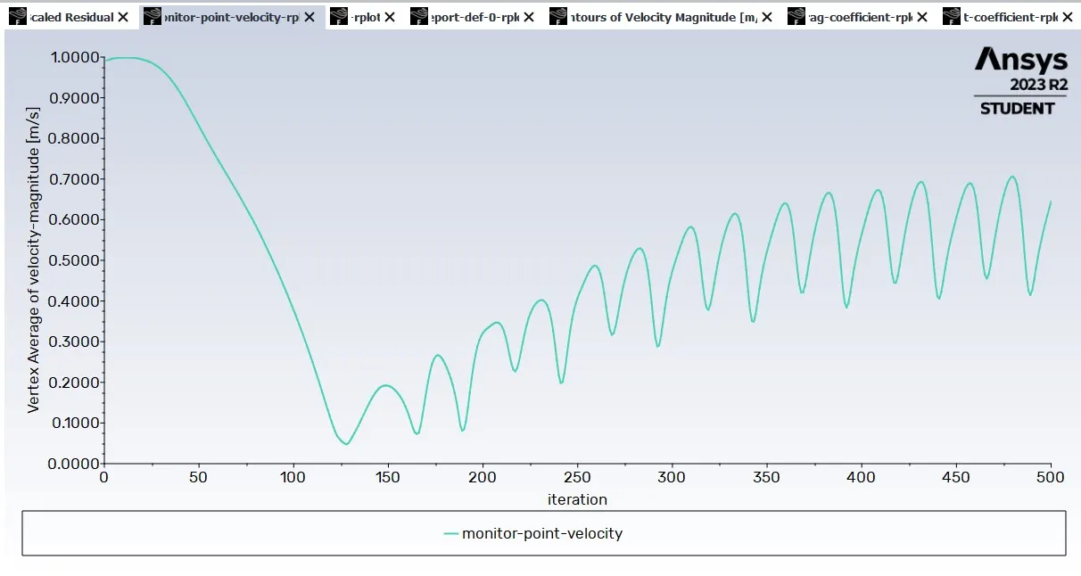
DRAG COEFFICIENT
LIFT COEFFICIENT
POST PROCESSED VELOCITY CONTOUR PLOT WITH VORTEX SHEDDING
UNSTEADY STATE ANALYSIS
When Reynolds number Re = 100
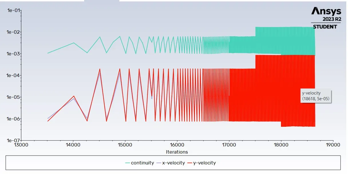
SCALED RESIDUAL
MONITOR POINT VELOCITY
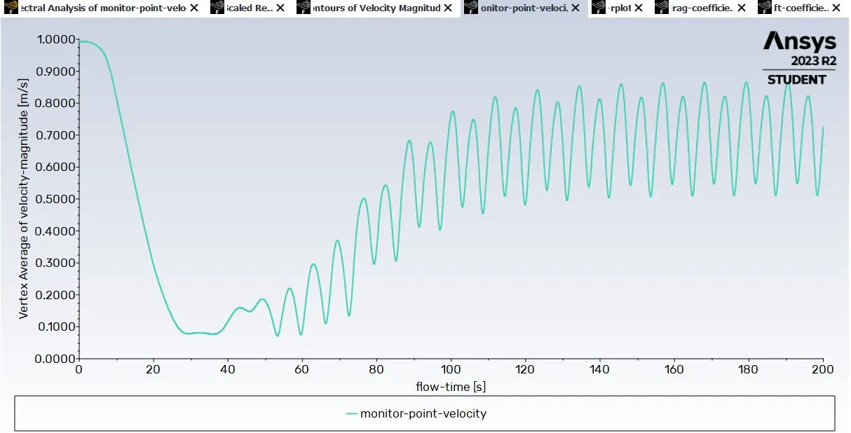
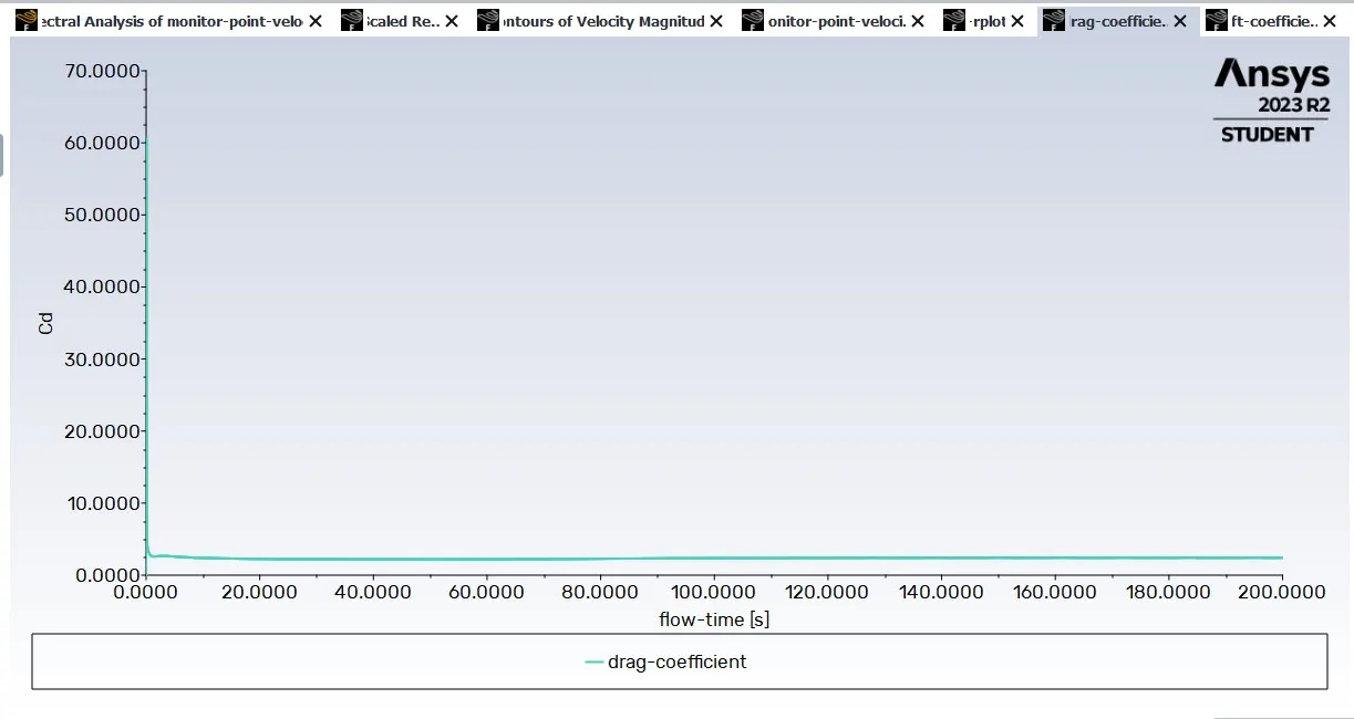
DRAG COEFFICIENT
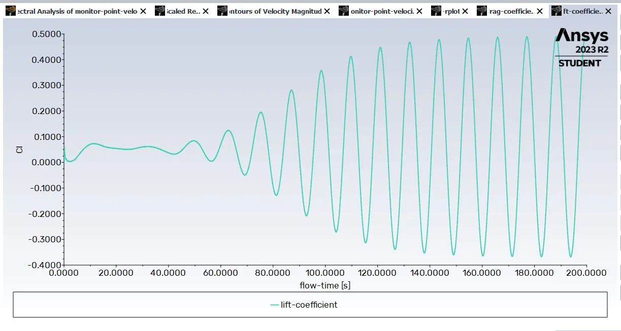
LIFT COEFFICIENT
VELOCITY CONTOUR PLOT
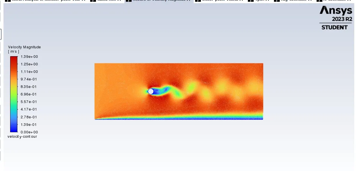
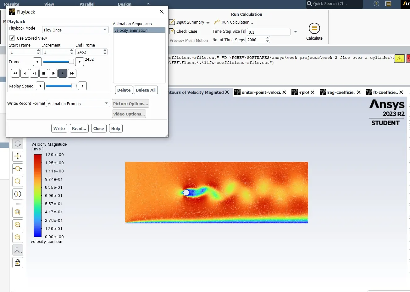
Unsteady state Inference
Here unlike the steady state the time factor has been used as the unsteady state works on time dependency of the flow. The time scale has been set for 2000 time steps with 0.1 of the scale as the time scale size. The simulation for this procedure took around 3 hours to complete and achieve the stable convergence of the flow.
STROUHAL NUMBER
Strouhal number relates the frequency of the vortices shedding through the monitor point , Spectral analysis of the flow flowing through the monitor point is defined
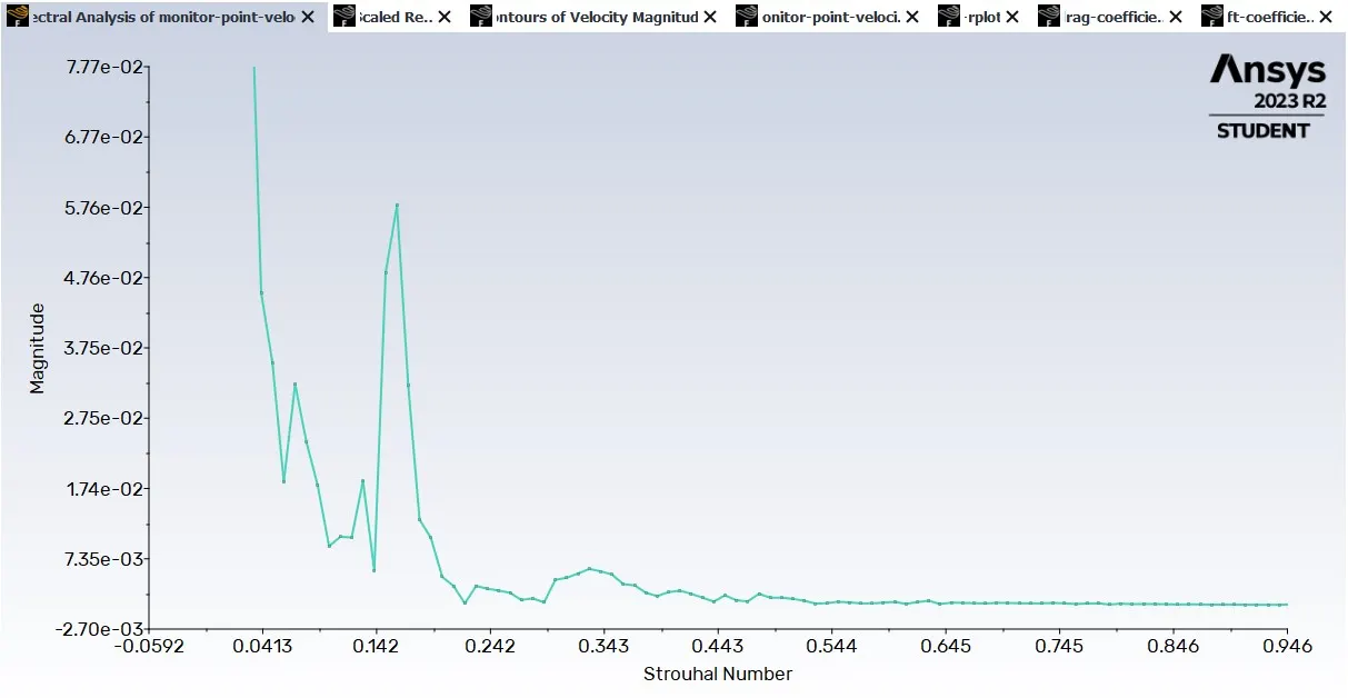
St = 0.161 peak achieved at monitor point
Strouhal number ,
- The frequency at which the vortices are shedding are proportional to the velocity of the flow and inversely proportional to the characteristic length of the material , In this case a cylinder is used (so L=d)
f = st.U/d
where st is the strouhal number.
- If Strouhal number is high then the oscilations produced from the flow would dominate the flow stream and if the Strouhal number is low then the oscilations are swept away by the flow stream.
PART 2
Calculating the drag coefficent and lift coefficient over a cylinder for the flow flowing through it when Reynolds number
(Re =10,100,1000,10000 and 100000) in a steady state solving condition.
Reynolds number =10
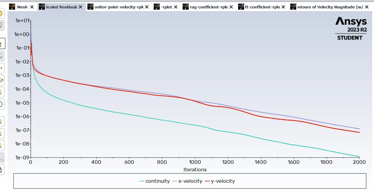
SCALED RESIDUALS
DRAG COEFFICIENT
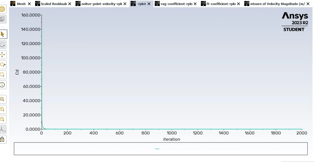
Cd = 0.0652
LIFT COEFFICIENT
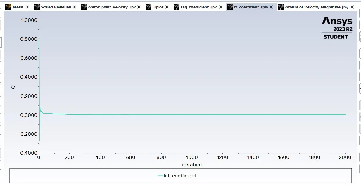
Cl = 0.0031
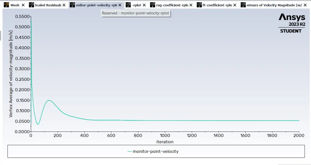
MONITOR POINT VELOCITY
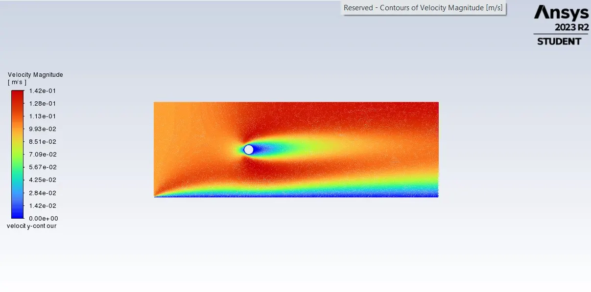
VELOCITY CONTOUR PLOT
Inference:
When Reynolds number is set to 10 by varying the stream velocity to 0.1 , density = 1 and dynamic viscocity to 0.02 , Vortex shedding is never achieved after 2000 iterations in a steady state condition . This is due to low Reynolds number value.
Reynolds number = 1000
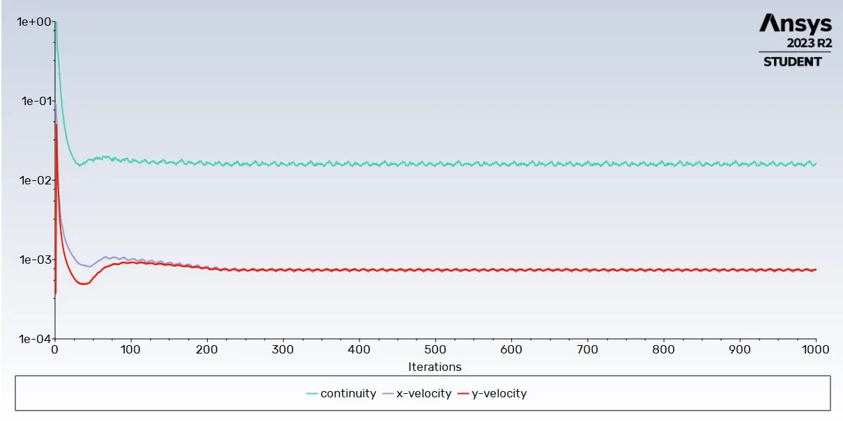
SCALED RESIDUALS
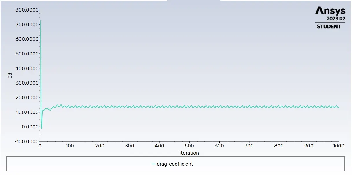
DRAG COEFFICIENT
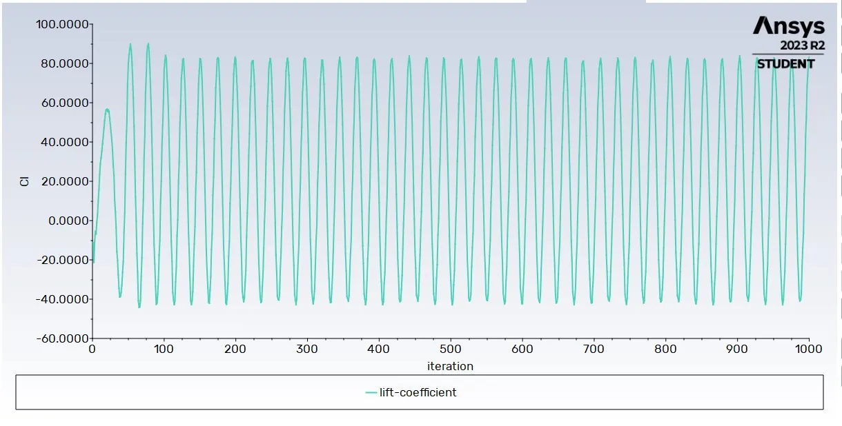
LIFT COEFFICIENT
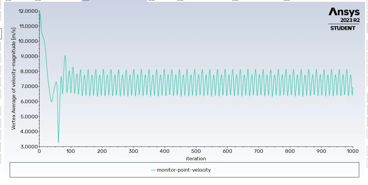
MONITOR POINT VELOCITY
VELOCITY CONTOUR
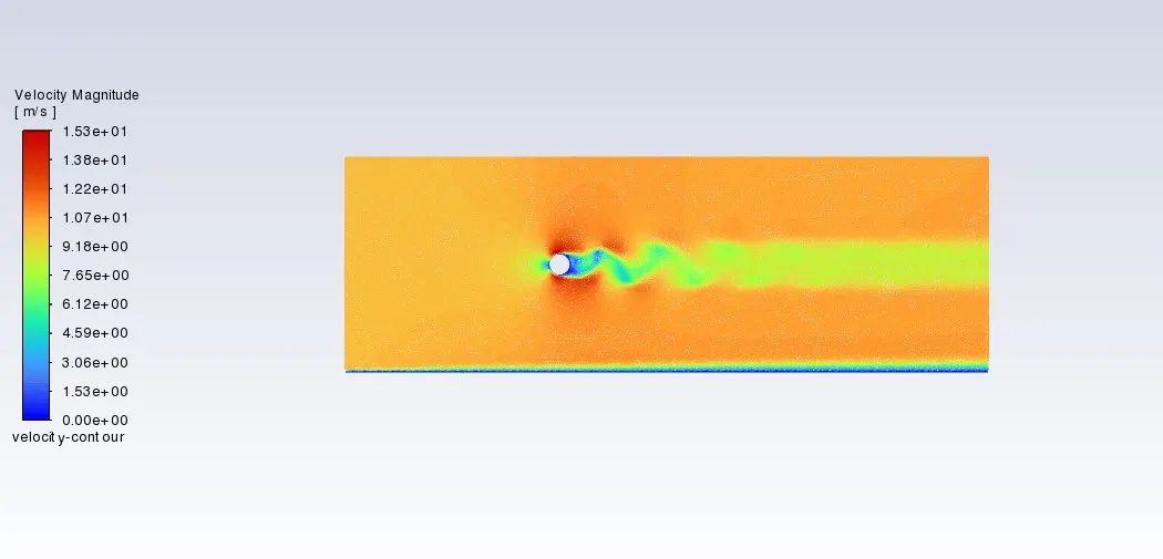
Inference:
When Reynolds number is set to 1000 , The vortex shedding occurs at a frequent rate and the lift coefficient and drag coefficient corresponds uniformly for the steady state solving condition.
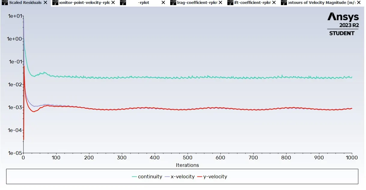
When Reynolds number = 10000
SCALED RESIDUAL
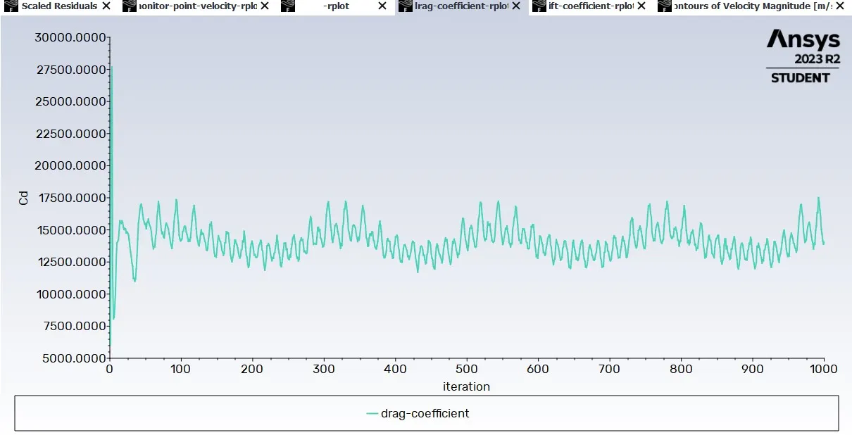
DRAG COEFFICIENT
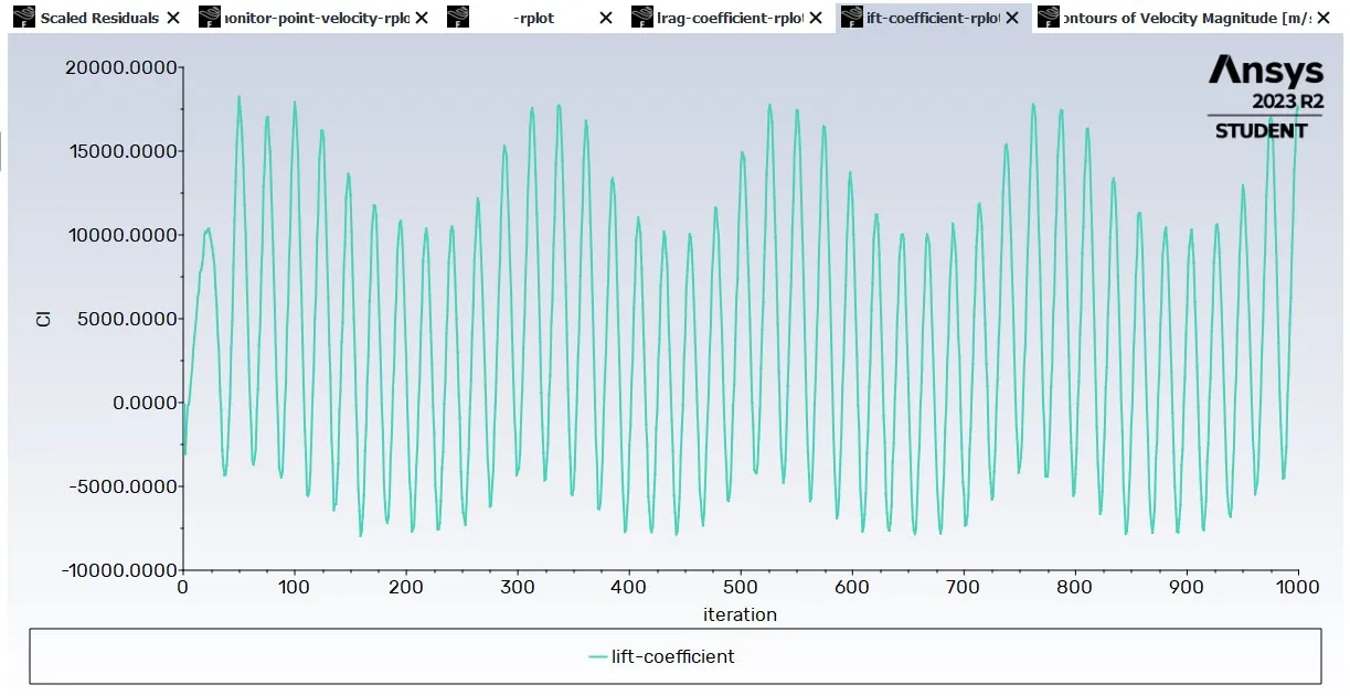
LIFT COEFFICIENT
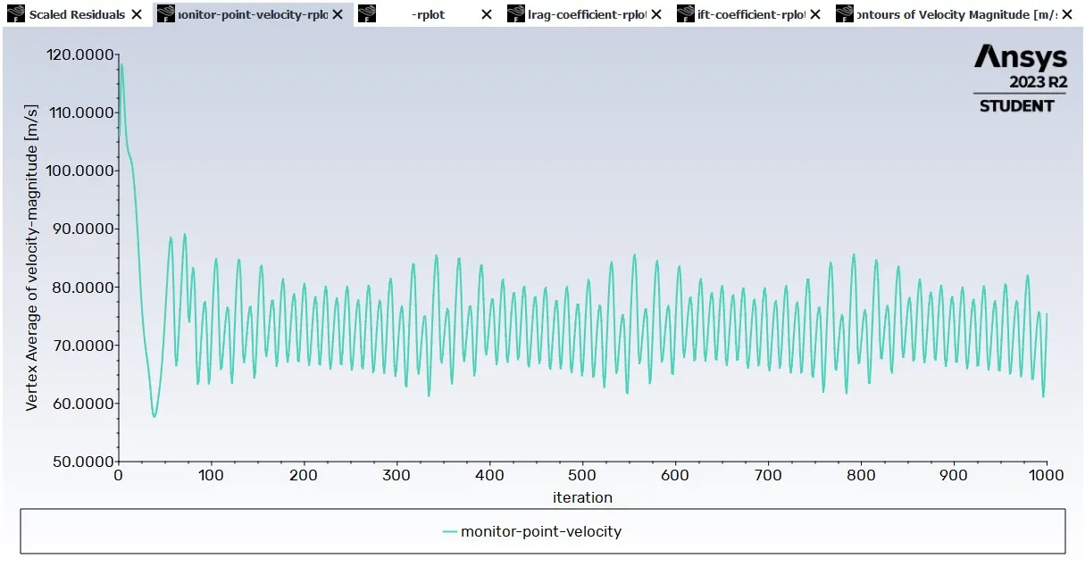
MONITOR POINT VELOCITY
VELOCITY CONTOUR
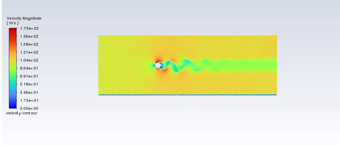
Inference :
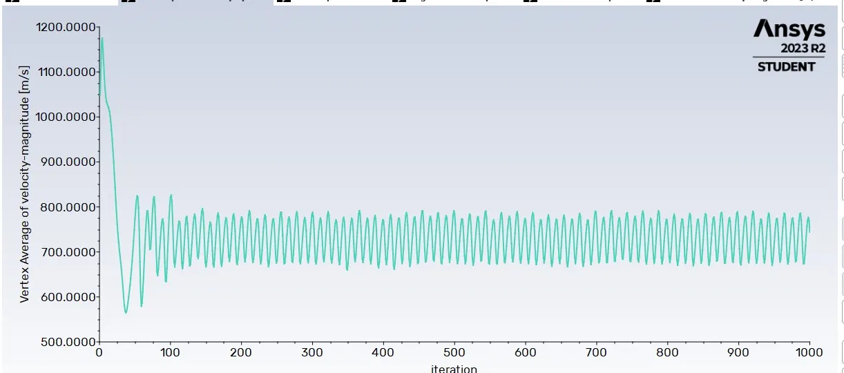
When the Reynolds number is set to 10000 by changing the velocity of the stream flow to 100m/s , density = 1 and dynamic viscosity to 0.02 , Vortex shedding happens at a higher frequent rate following a set of patten , this could be seen in drag coefficient plot, Lift coefficient plot and in monitor point velocity . This uniform set of patternal frequency also occurs in certain frequency due to uniformal pressure difference and Friction drag caused at the boundary layer of the material approching the stream flow. This pattern follows for corresponding iterations and thus the steady state is achieved.
When Reynolds number = 100000
SCALED RESIDUALS
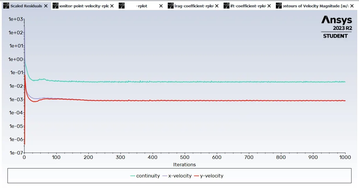
DRAG COEFFICIENT
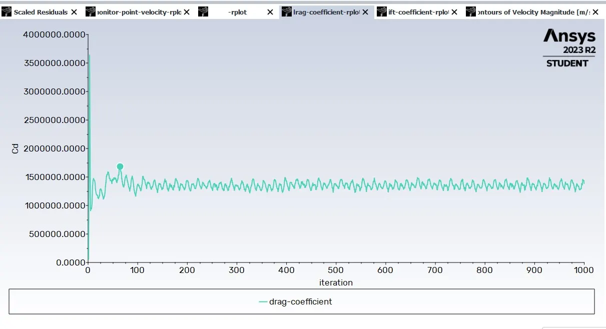
LIFT COEFFICENT
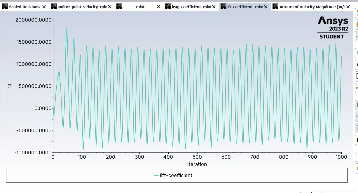
MONITOR POINT VELOCITY
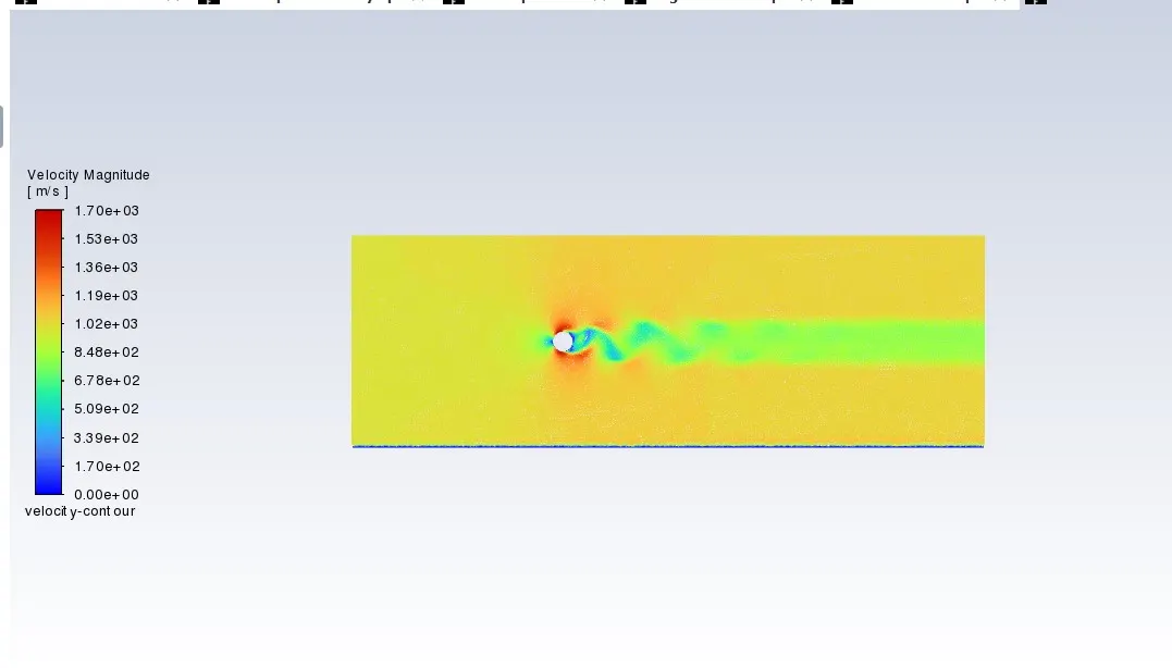
VELOCITY CONTOUR
CONCLUSION
|
REYNOLDS NUMBER (Re) |
Cd- drag |
Cl - lift |
|
10 |
0.0652 |
0.0031 |
|
1000 |
145.975 |
83.526 |
|
10000 |
17078 |
17750 |
|
100000 |
1475447 |
1436074 |
- As the Reynolds number increases, the flow velocity increases and as it increases , It corresponds to increase in drag coefficient and lift coefficeint of the flow
Research reviewed
https://www.sciencedirect.com/topics/engineering/strouhal-number