Week 2 - Flow over a Cylinder.

Aim:

The objective the project is to simuatae the flow over the cylinder for the steady state & unsteady state conditions. The simulation will be carried out for various Reynolds number.The simulation will be carried out in the ansys Fluent workbench. For thr first simulation will be carried out in the ansys fluent workbench, For the frist part simulaton for Re100 in steady & unsteady conditions &strouhal number need to be calculate for Re 100. For the second part of the challenge is to calculate drag and lift coefficent for the flow over a cylinder for seriess of reynolds number 10,100,1000,10000,100000. the steady state simulation has been used for the second part.

Introduction:

The simulation of flow over the cylinder is very challenging for the reseracher till today. This simulation is very useful to understand the complex behaviour of fluid dynamics. Some of the applications are to understand the unsteady dynamics of wake flow behind the cylinder, cross flow normal to the stationary cylinder & the problem related to the mass & heat tansportations. this problems are related to wide variety of problem faced by the engineering feild.

The two most important phenomena associated with this type of simulations are vorex shedding & kamran vorex street.

Vorex shedding

It is a phenomena when the flow crosses the bluff body, vortices are shed alternately from one side to other. Where alternating low-pressure zones are generated to the downside of the bluff body giving rise to fluctuating force acting at right angles to flow direction.

Von Kamran Vorex Street:

The vortices which are sheded alternately frm either side of the bluff body & it creates the pattern of swirling vortices. These pattern of swirling vortieces are periodically & its called as von kamran vorex street.

Depends on the force, the body might move towards the direction of the force. If the bluff body doesnt mounted rigidly on the stracture than it will start vibrating with hormonic oscillations driven by the energy of flow & if the vorex shedding frequency of the vibration reaches the frequencey of structural-vibration frequency of the body start resonating. This phnomenon is major importance in engineering design because the alternate formation and shedding of vortices also create alternating forces, which occur more frequently as the velocity of flow increases.

When the frequency is in the audible range, a sound can be heared and the body appears to sing. many struturures failled because of phnomena. Beacause of this effect, it isvery important to study the vorex sheding to make sure performance of the components will not affect by the vorex shedding.The strouhal number has been used while studying this type of phenomena.

Strouhal Number(sr or st):

This is a dimensionaless number which used to a measure of vorex shedding frequency. This number is function of Reynolds number but less of surface a roughness & freestream turbulence.

Sr=fL/U

f=frequency of vertex sheading

L=Charectristic length

U=Flow velocity

Design inputs:

Material : Air

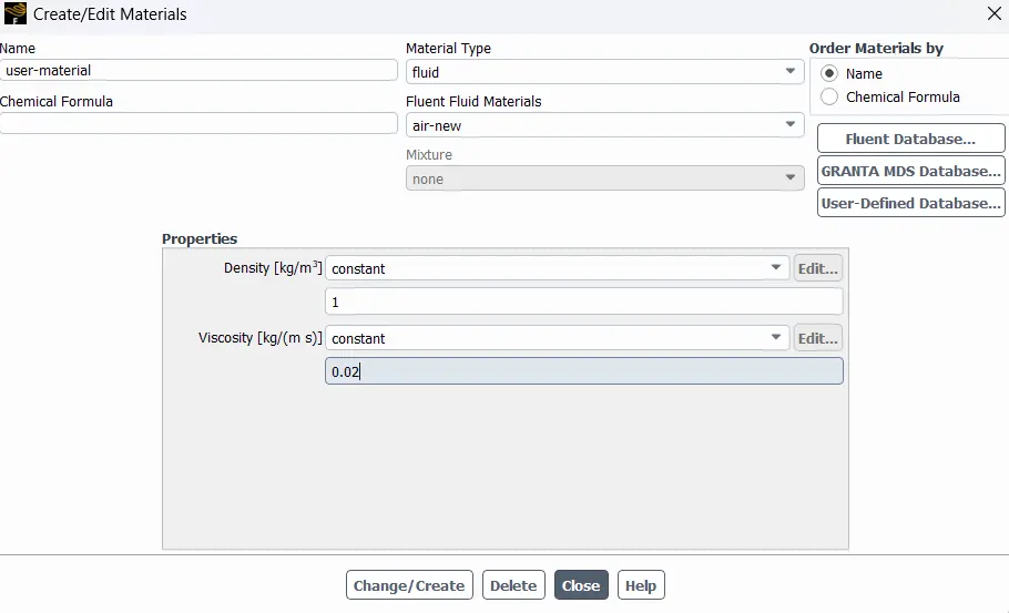
Density : 1 kg/m^3

Viscosity :0.02Ns/m^2

Gomentry Creation:

• From this point, we can start our project by creating our gomentry in spaceclaim using given dimensions.
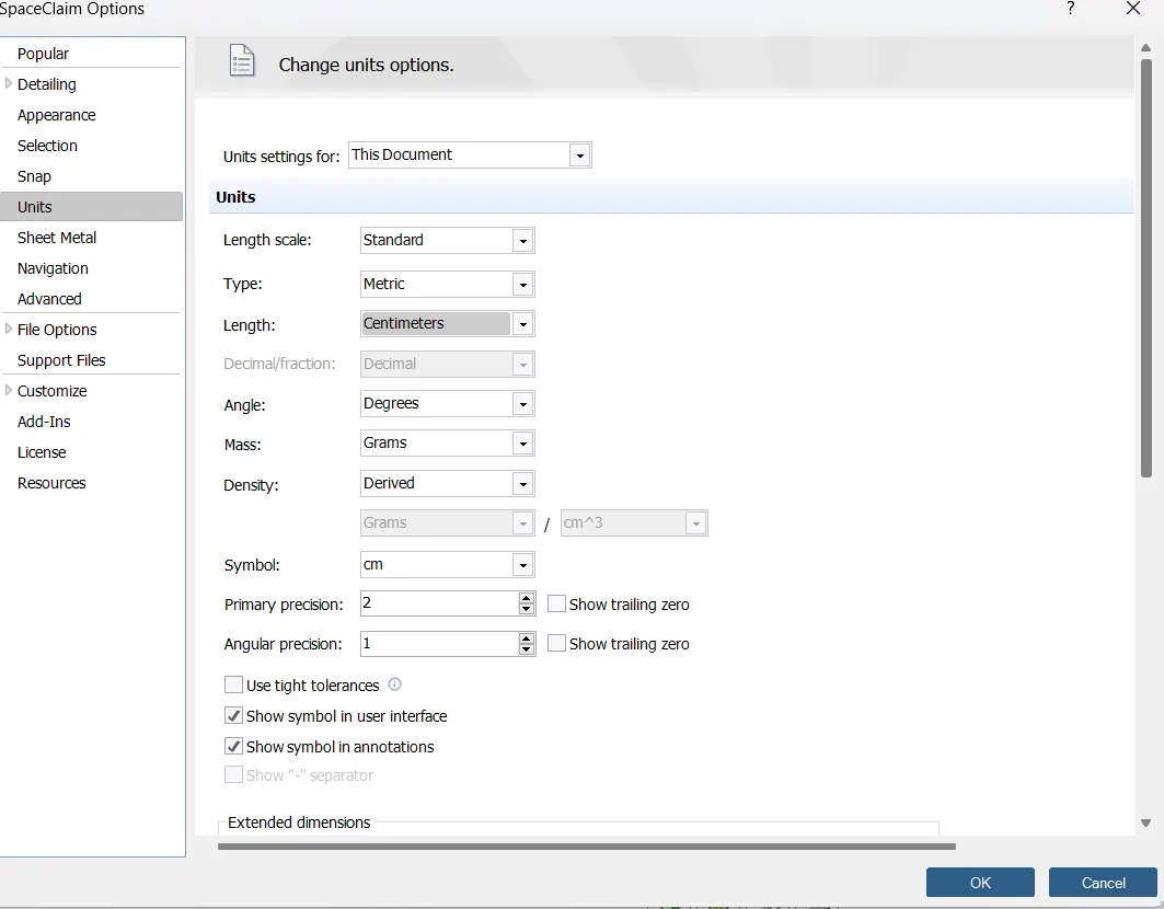
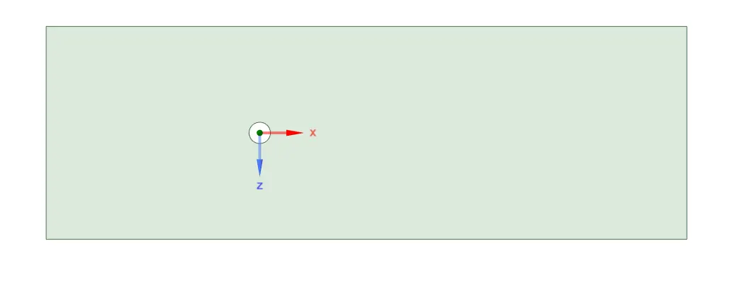
• After open the spaceclaim, using the the circular dimension is 2m. Circle to the inelet at the distance 20m and outlet is 40m. Symmetry boundary conditions are 10m apart from the center of cylinder.Size of the computational domain is 20*60.

Meshing:

• Now click on mesh in workbench to open mesh.
• In the mesh right side in top project to click the mesh-right click-generate mesh.To do this we have to no how the mesh from in 2d domain.

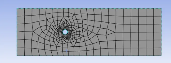
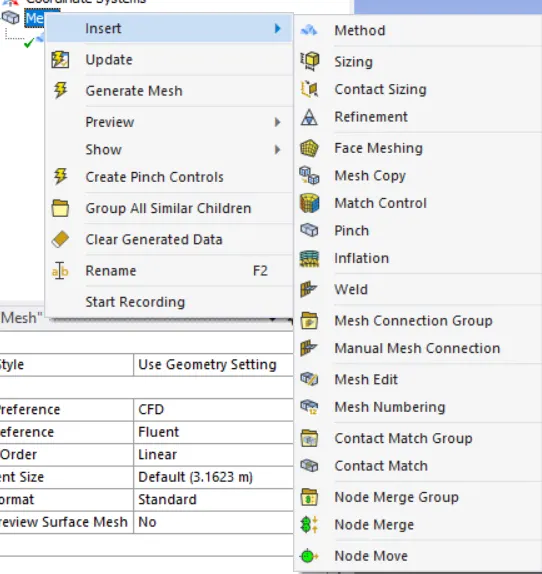
• Intially the mesh is generating in qudra mesh to improve the mesh quality and change the qudra to tria.In the mesh to using insert option to create the Method and select the required surface and method to change the quadra to tria in mesg to generate.

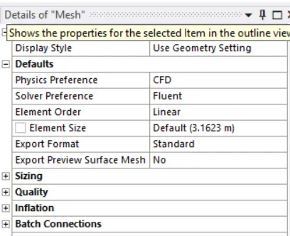
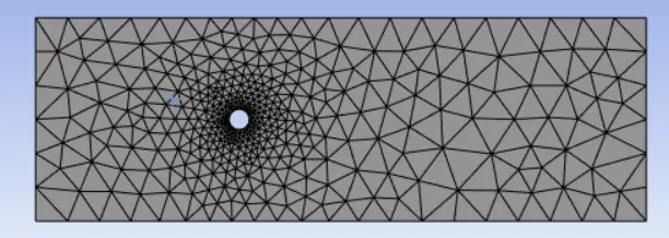
• After genrate the tria mesh to look the cylinder the shape of the cylinder is converted shape.To inser the sizing using the egde tool to select the circle and type is converted to number of divisions.

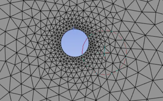
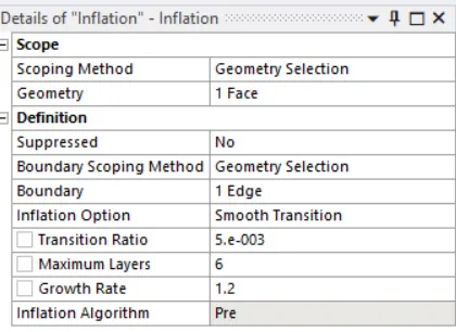
• Infulation layer:Inflation layers are inflated from a triangular surface mesh to create high quality geometry aligned elements capable of resolving boundary growth.
• It is a thin element near the wall thet capture the normal gradient of velocity and temerature.
• influation layer thickness:First iflation layer hight have chosen is 5mm and the maximum layer are 6 and the growth rate is 1.2. Which means each inflation layer thickness is increasing 20%.

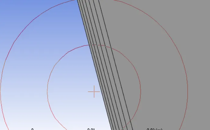
• After generate the mesh using the edge selecter to select the required edge create names.

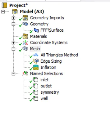
Simulation Setup:.

• For stedy state.
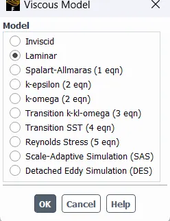
• We select a laminar option in the viscous because Reynold number is low. Re changes with change in flow velocity or by changing the fluid that means dynamic viscosity.

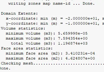
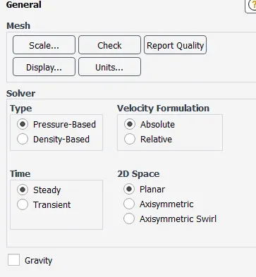
• Now the material is user -material to crate and assign the density 1 kg/m^3 and viscosity is 0.02 kg/m-s.

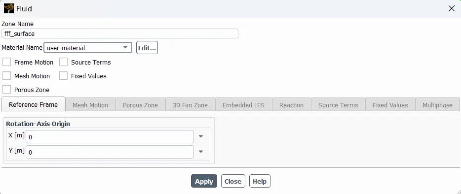
• Cell zone to open and volume to assign the matrial we are created.

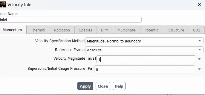
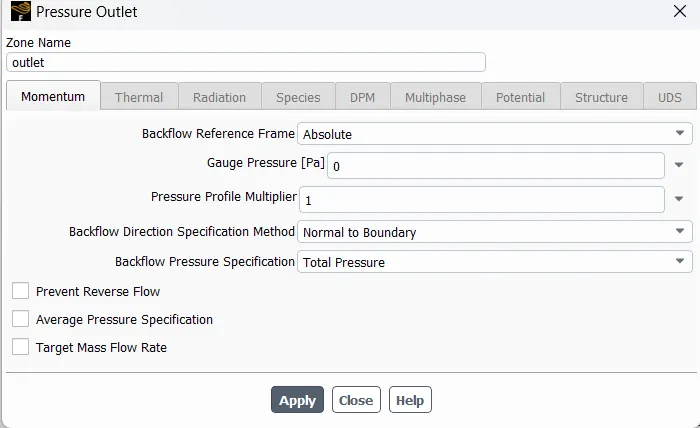
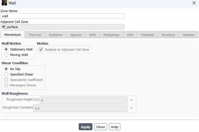
• The inlet velocity id defined as value corresponding to Reynold's number. The outlet Bc is pressure type with gauge pressure equal to zero,as it is open to the operating condition (atmosphere). These along with wall boundary conditions of no-slip for cylindr wall and symmetry BC are assigned in the boundaries option of the zones section. 

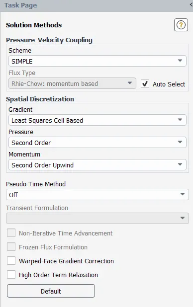
• open the solution domain and method to set to be second order and schem to change to simpe mode.

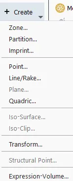
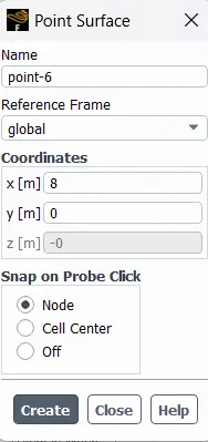
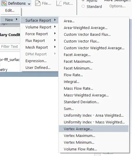
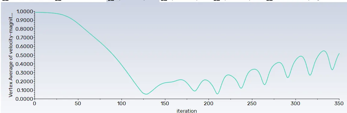
• To create the moniter point in the domain using point option.Then go to the defnition to create new to surface report create vorex average.

                                 

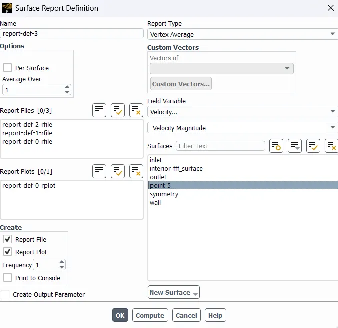
• Vorex average to chnge the varible to velocity select the monito point to create the report file and report plots.

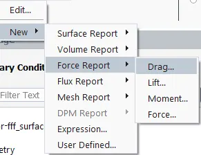
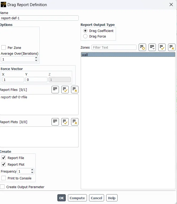
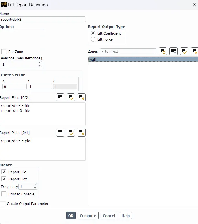
• After setting all the above setup condition, initialization of domain has be done neccessary, because the solution is an iterative process that can be executed if there is an intial guage of solution varible.
• Inthis case we use the hybrid intialization and click the intialization.

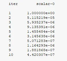
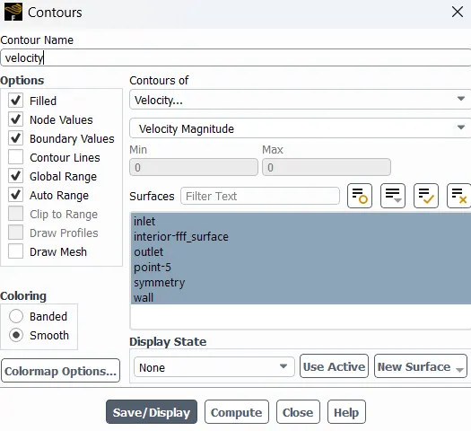
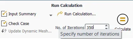
• Go to the run calculation setup the number of iteration and calculate.

Results:

Part1:

Simulation of flow for the steady condition for Re=100

st=fl/U

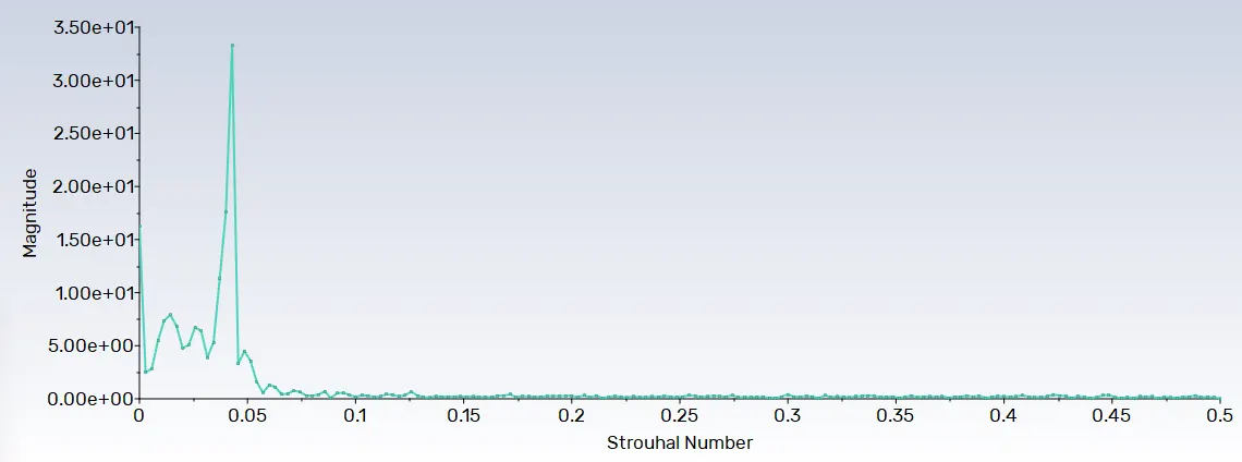
f=number of cycles /time=3/30=0.1

St=(0.1*2)/1=0.2

Steady state:

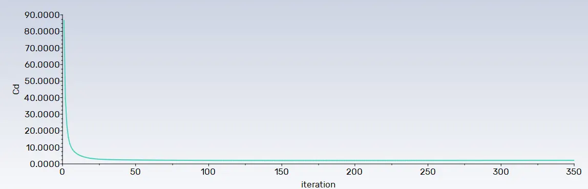
Unstedy state:

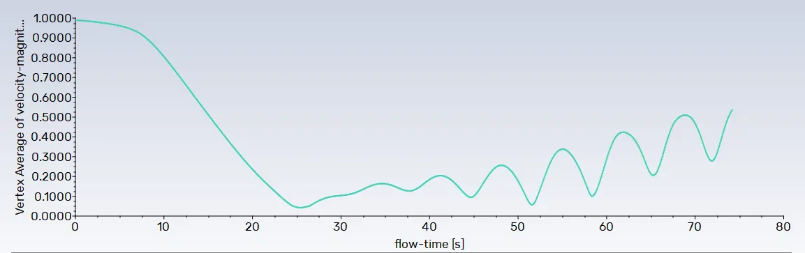
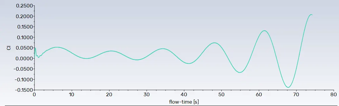
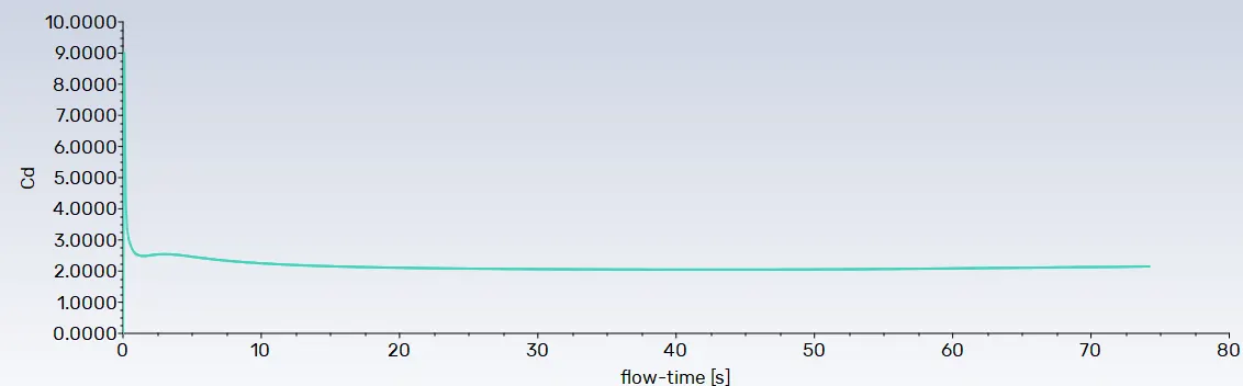
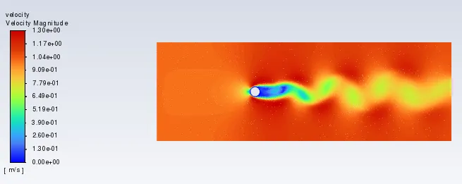
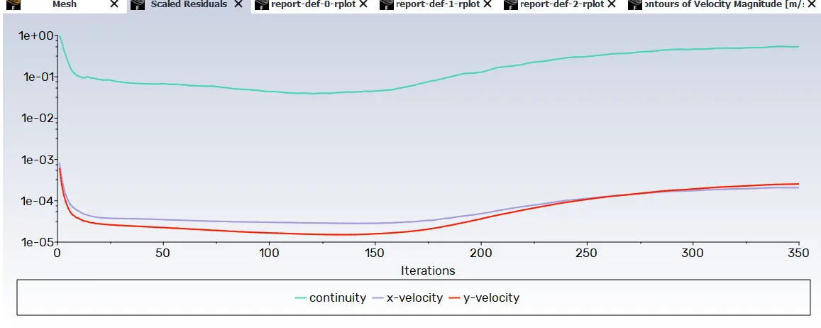
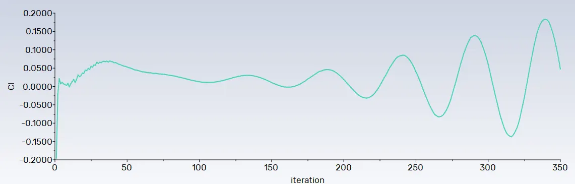
From above images follwing observation can be made.

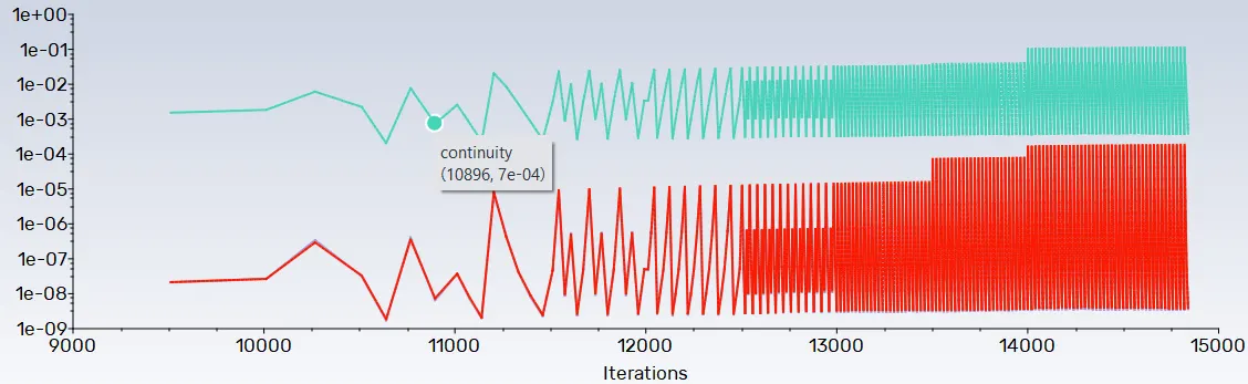
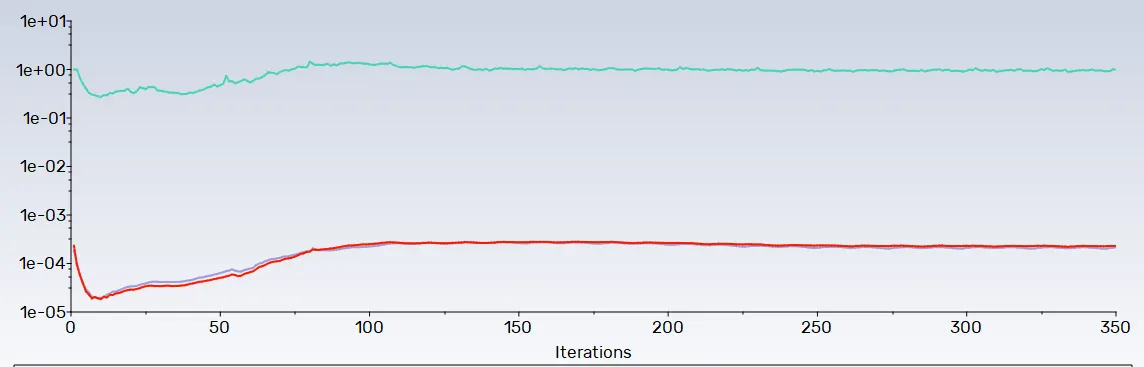
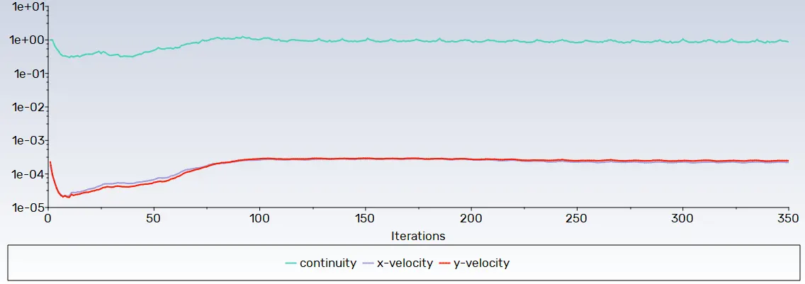
• In residual plot, the error value is neither changing not increasing from the set limit of Le-3, that's why it can be said that solution is converged.
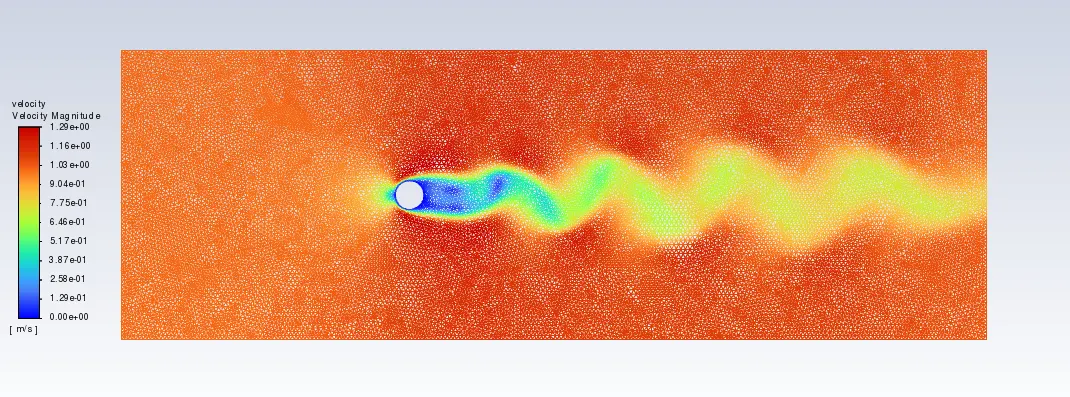
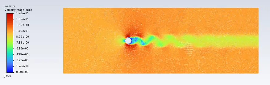
• In velocity contour plot, the von kamran vorex steet can be seen.
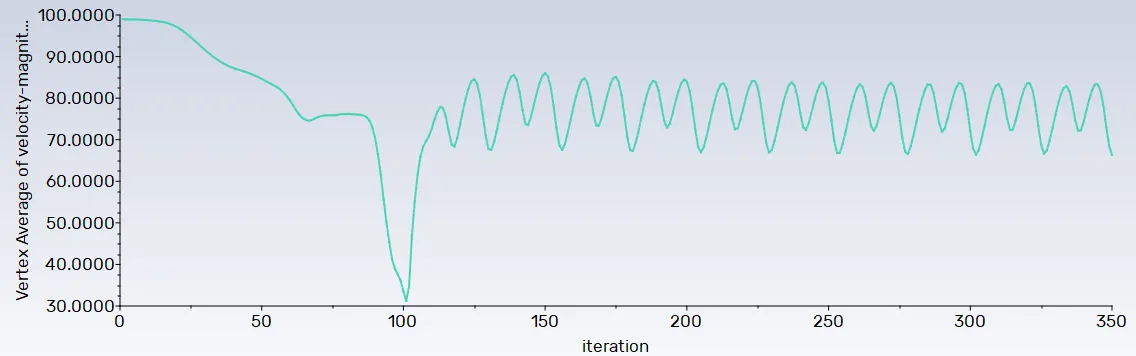
• In the lift contour plot, the value is kept rising & faling because of vorex shedding phenomena. The lift coefficient data has been used in fourier transfrom (FFT) plot to plot the strouhal number.
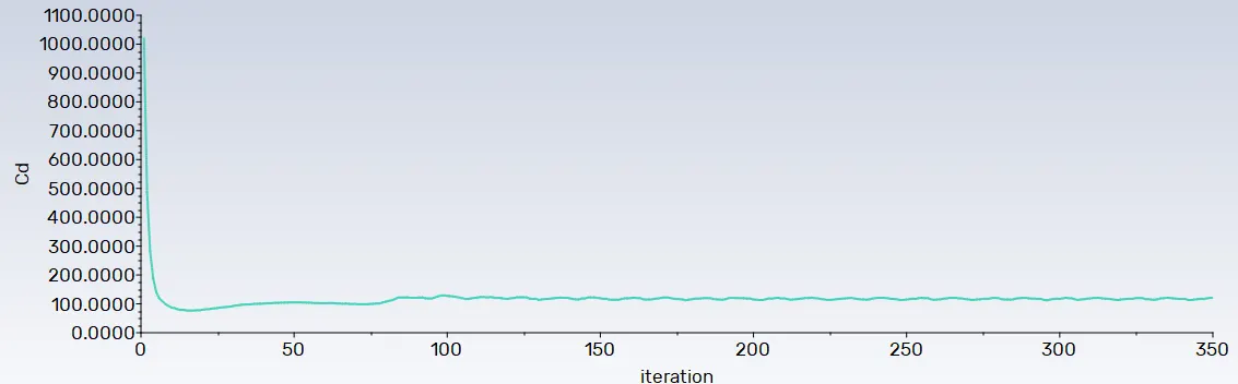
• The drag coefficent value is constant after one point. The drag coefficient of cylinder is calculated by the fluent is around 1.33.
• The drag coefficient value has been compared with the expermental data provided in the follwing paper written by B.N.Rajani which is  "numerical simulation of lamiar flow past a circular cylinder". The drag coefficient values are within the 5% variance in comparison with the expermental data.

Part2:

where 

Re=Reynolds number

ρ  =density

U=flow velocity

L=characterstic length

μ=Dynamic viscosity

Density                           1            kg/m^3

characterstic length         2                 m

Dynamic Viscosity        0.02            kg/m s

Reynolds Number          Flow velocity          units

10                                     0.1                   m/s

100                                     1                    m/s

1000                                  10                    m/s

10000                                100                  m/s

100000                              1000                 m/s

For Re=10

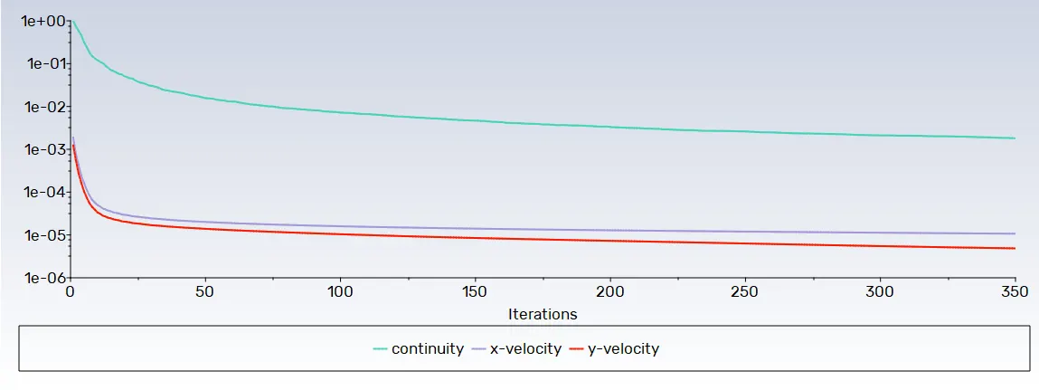
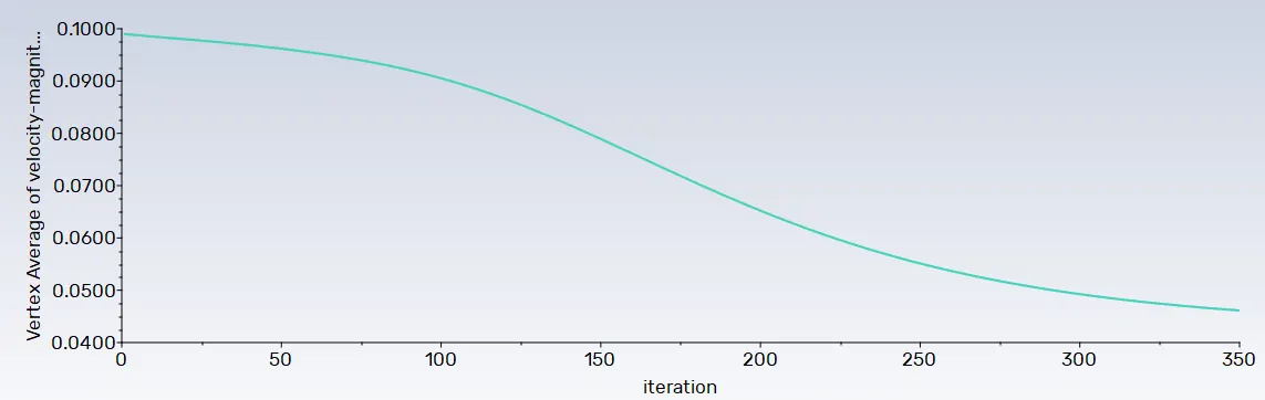
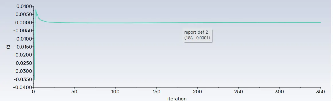
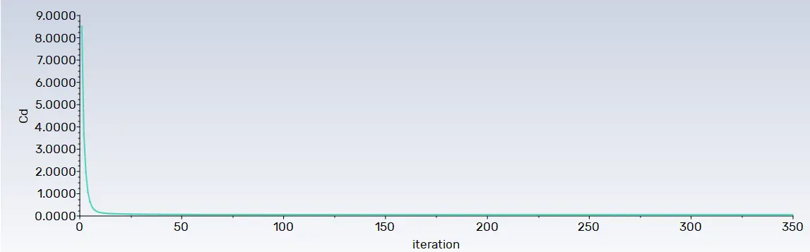
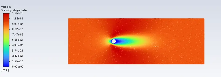
For Re=1000

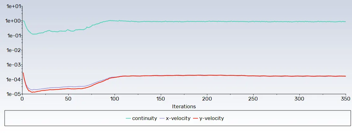
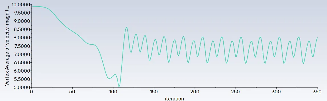
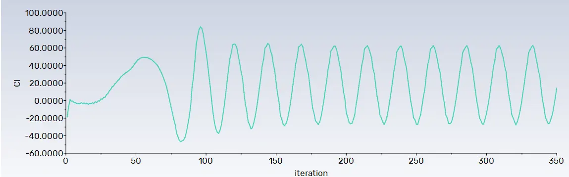
For Re=10000

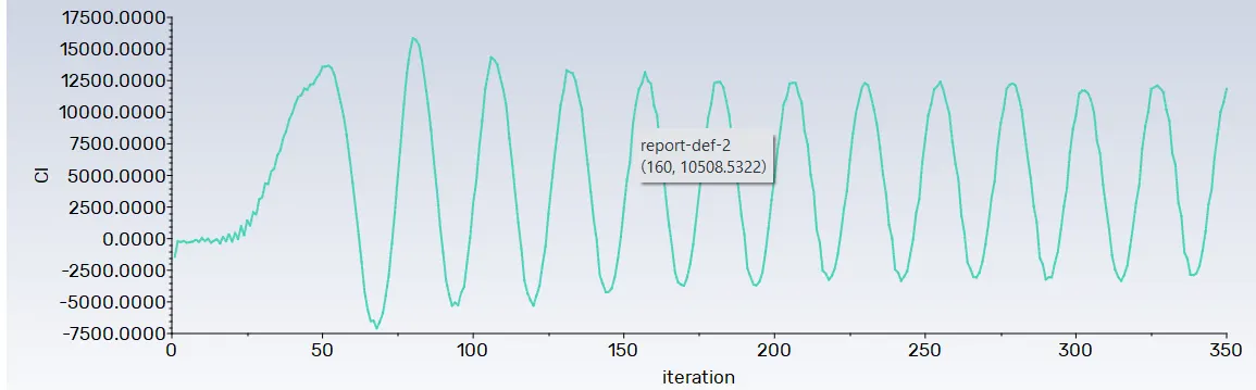
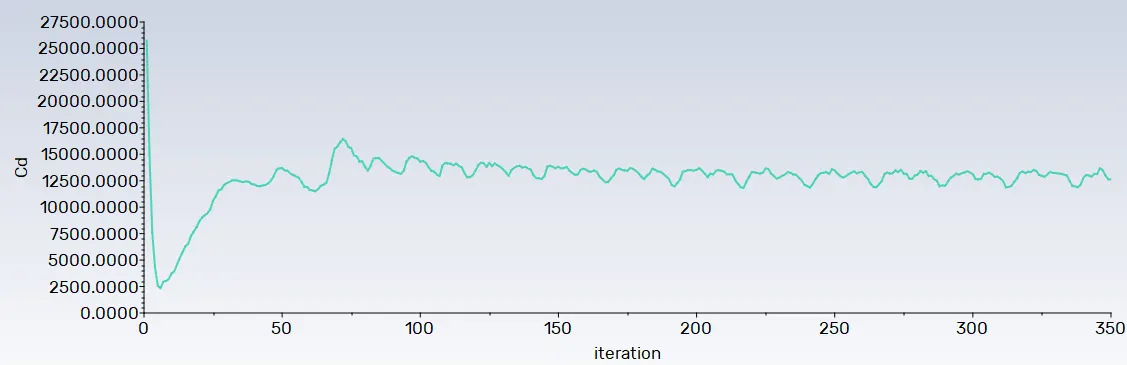
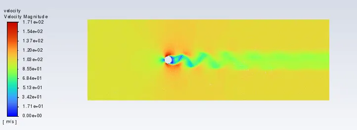
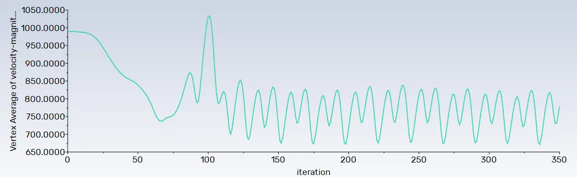
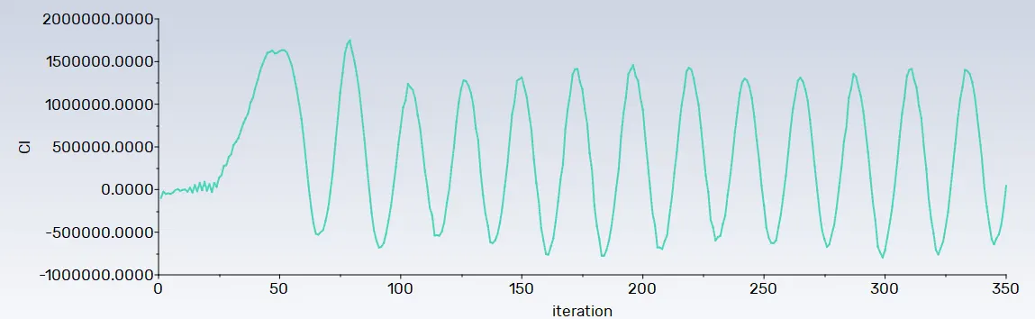
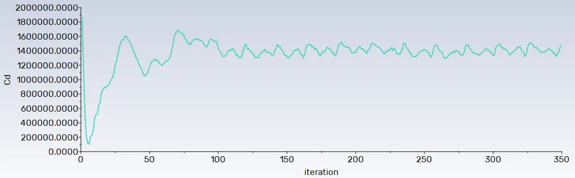
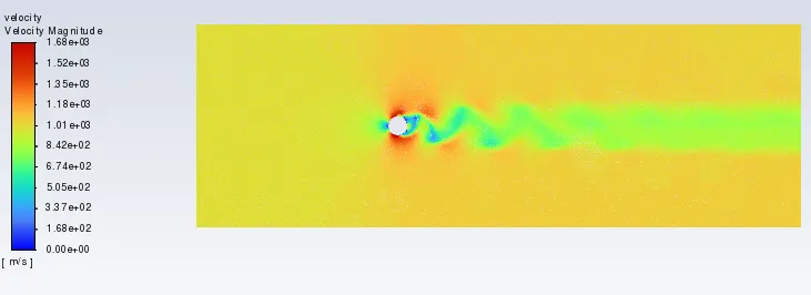
For Re=100000

Conclusion:

The time & resoures consumes by the transient solver is for more than steady state solver.

For the transient simulation , the simulation were running off the convergence criteria. In this transient mose, the more iteration are required to develop proper physical of the flow. Because of the transient simulation has taken more iteration with smaller time compared to the steady state.

The drag coefficent for the Re above 1000, is start fluctuating but perodic after one point which can be seen from the results images. So statically, it is constant.

The results of simulations are the one we are expecting from the physical point of view.

The challenge of simulating folw over a cylinder has been carried out to study the vortx shedding phenomena & visualizing von kamran vorex street. The challenge has been divided into two parts. In first part, the stedady & unsteady state simulation have been perfromed for Re 100 & stouhal number has been calculated using analytical method & later compared with the fluent result. While in second part series of simulation has been carried out for various Re numbers in stedy state consition. Vortex shedding & kamran vorex street was unable tovisualize for Re 10 because these two phenomena doesnt occur below Re 40. The drag coefficent & lift coefficent has been compared for all simulation

References:

1.Numerical simulation of laminar flow past a circular cylinder- https://www.sciencedirect.com/science/article/pii/S0307904X08000243

2.Flow regimes-

 https://www.sciencedirect.com/science/article/pii/B9780123815293000049

3.Strouhal number-https://www.sciencedirect.com/topics/engineering/strouhal-number#:~:text=Strouhal number is defined as,is the free-stream velocity