Week 2 - Flow over a Cylinder.

Flow Over a Cylinder:

1) Aim :

- Simulate the flow over the cylinder and explain the phenomenon of Karman vortex street.
- First, simulate the flow with steady and unsteady cases and calculate the Strouhal Number.
- Second, calculate the coefficient of drag and lift over a cylinder by setting the Reynolds number to 10,100,1000,10000 & 100000(run with
steady solver)
- Then, discuss the effects of the Reynolds number on the coefficient of drag(results should be validated with any standard literature and
the error should be within 5%)
- In both approaches show that the flow has converged. Mention the quantities or plots which determine that the flow has converged.
- Plot the coefficient of drag and lift.

3) Introduction :

• Flow over a cylinder is important in many industrial applications like cooling of iron or cylindrical pipe
• Circular pipes have more application in the heat exchanger. High-temperature flue gases flow over a circular cylinder in a cross flow.
• Depending on flow rate, fluid properties, and size of cylinder, the flow can be laminar, transition and turbulent

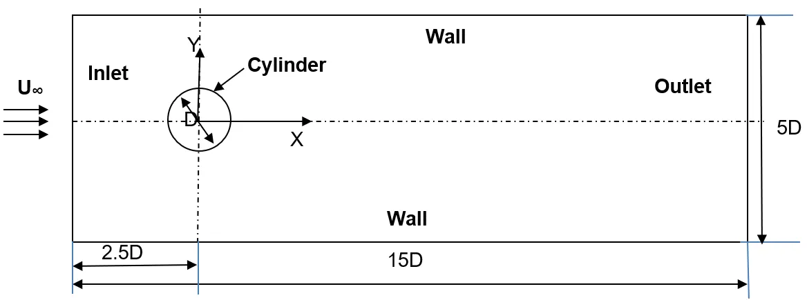
4)Theory :

The Reynolds number is a key parameter in fluid dynamics. It describes the fluid, geometry, and flow. This allows us to compare different fluid systems. It is the measure of the ratio of inertial to viscous forces in the flow of a fluid and is defined as,

Re=ρ⋅D⋅U/μ

where,
ρ = Density of the Fluid
U = Inflow Velocity
D = Diameter of Cylinder
μ = Dynamic viscosity of Fluid

As we increased the flow rate(and Reynolds Number), the flow develops into a variety of structures. After a particular value of Reynolds number, the flow becomes unstable resulting in a moving wake, famously known as Karman vortex street. These increases drag.

5)Procedure :

PART-I

1. Simulate the flow with the steady and unsteady case and calculate the Strouhal Number for Re= 100.

PART-II

1. Calculate the coefficient of drag and lift over a cylinder by setting the Reynolds number to 10,100,1000,10000 & 100000. (Run with steady solver)
2. Discuss the effect of the Reynolds number on the coefficient of drag. [ Results should be validated with any standard literature and error should be within 5 %]

GEOMETRY --> MESHING --> SETUP & SOLUTION --> RESULT.

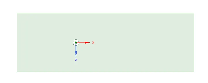
5.1) Geometry Creation :

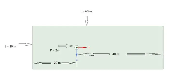
5.2) Meshing :

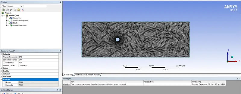
The generated 2D geometry meshed with an element size of 6mm(here ia am using some higher mesh length due to system limitation, But less mesh size is only preferable for increasing accuracy). The mesh was generated and proper inflation layers are given around the cylinder all to capture the wall boundary with a growth rate of 1.1. The number of the generated elements is 7262

5.3) Setup and Solution:

Setup parameters :

• Viscous model	Laminar
  Solver type	Pressure bases
  Solving Scheme	SIMPLE
  Initializing methods hybrid	Hybrid(for Steady case) Standard(for Transient case
  No. of Iterations	350

Case A) At Re = 100,simulate the flow with steady and transient method and calculate the Strouhal number.

• Material - User defined fluid with rho = 1kg/m^3
• ρ= 1kg/m^3
• μ=0.02 kg/m-s
• U = 100*(0.02/1)/2=>U=1m/s

A1) Steady Case

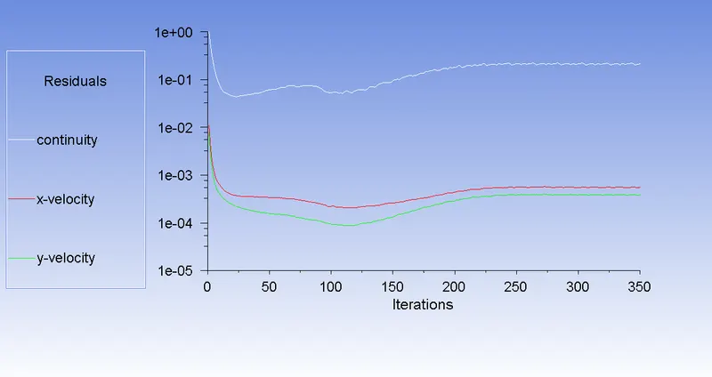
Fig - Residual Plot For Re = 100(Steady)

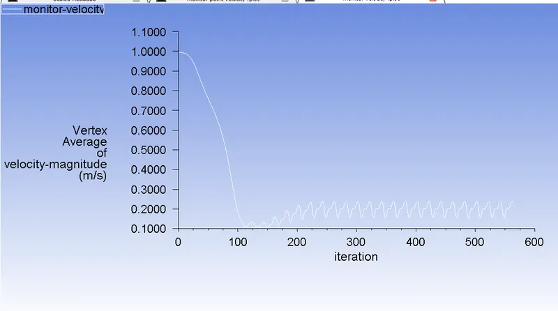
Fig - Vertex Average of Velocity Magnitude Plot For Re = 100(Steady)

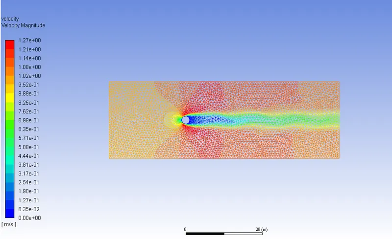
Fig - Velocity Contour For Re = 100(Steady)

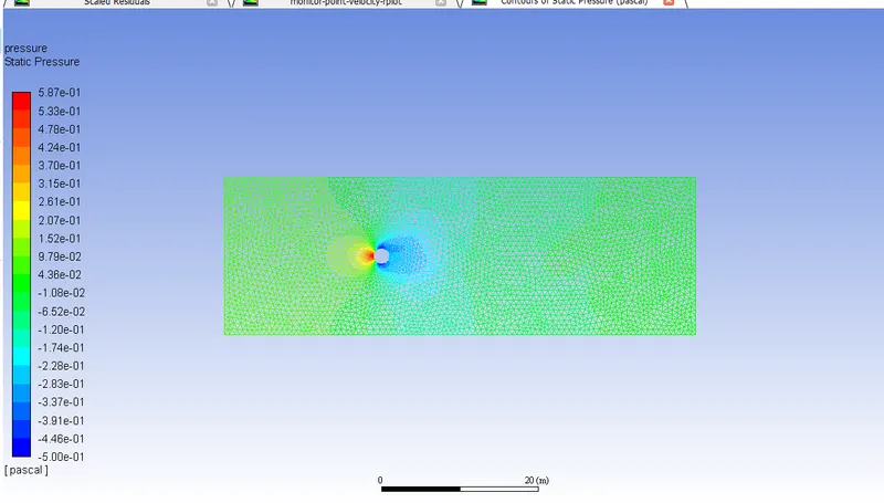
Fig - Pressure Contour For Re = 100(Steady)

A2) Transient Case:

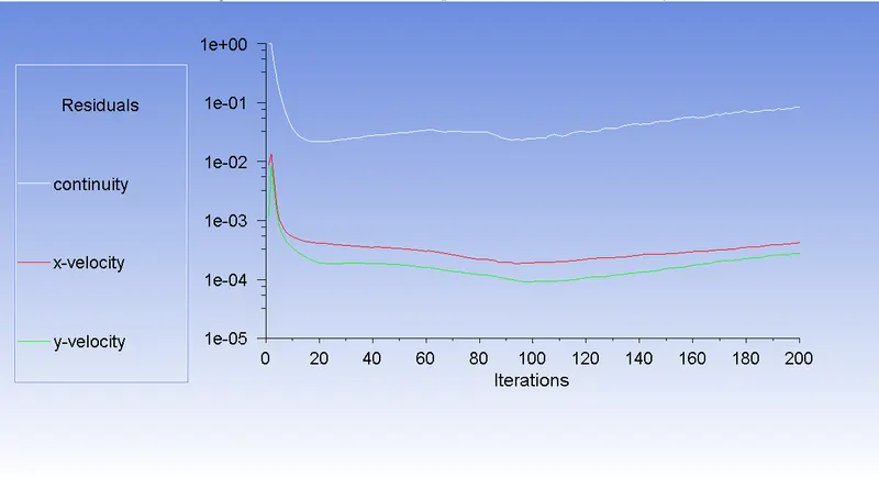
Fig - Residual Plot For Re = 100(Transient)

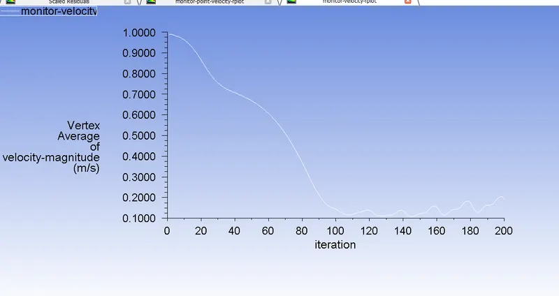
Fig - Vertex Average of Velocity Magnitude Plot For Re = 100(Transient)

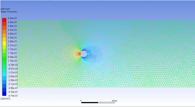
Fig - Pressure Contour For Re = 100(Transient)

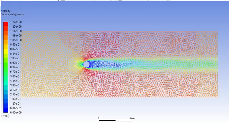
Fig - Velocity Contour For Re = 100(Transient)

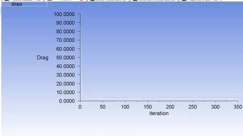
Fig - Coefficient of Drag Plot For Re = 100(Steady)

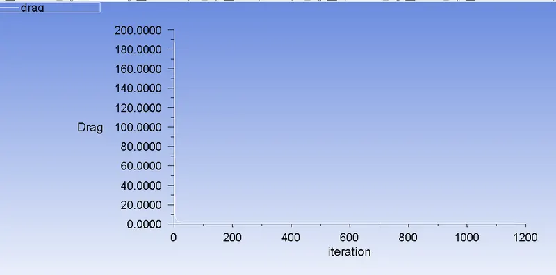
Fig - Coefficient of Drag Plot For Re = 100(Transient)

If we compare steady and transient cases concerning their drag coefficient, at steady state drag is almost constant after around 100 iterations. While transient, it is varying in a small frequency concerning time. Regardless both solutions are showing the same value of drag

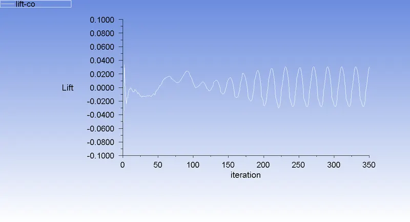
Fig - Coefficient of Lift Plot For Re = 100(Steady)

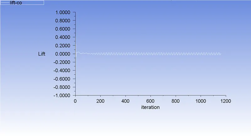
Fig - Coefficient of Lift Plot For Re = 100(Transient)

In lift plot,steady solution improving frequency from zero to approximately +-0.2. For transient, we see a repeating sine wave.

Strouhal Number:

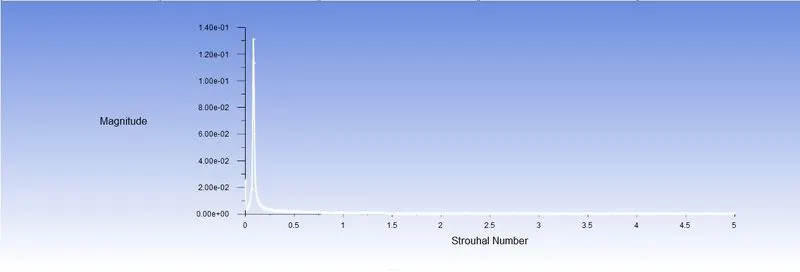
From the above plot of Strouhals Number and ,using highest value of magnitude Strouhal number was found to be 0.1.

Case .2

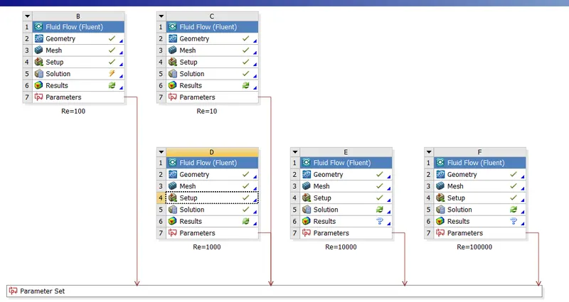
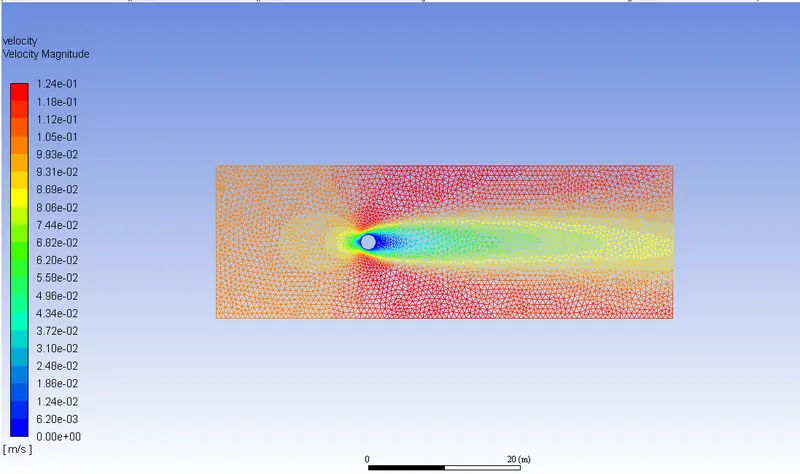
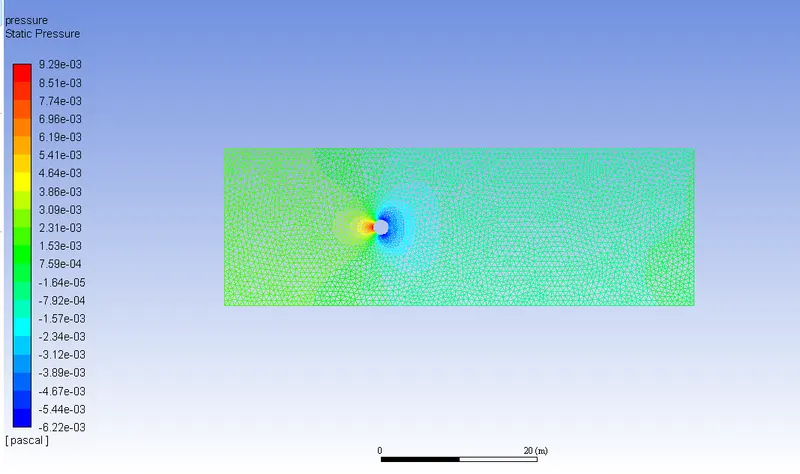
B1) At Re = 10,

• Material - User defined fluid with rho = 1kg/m^3
• ρ= 1kg/m^3
• μ=0.02 kg/m-s
• U = 10*(0.02/1)/2=>U=0.1m/s

B2) At Re = 100,

• Material - User defined fluid with rho = 1kg/m^3
• ρ= 1kg/m^3
• μ=0.02 kg/m-s
• U = 100*(0.02/1)/2=>U=1m/s

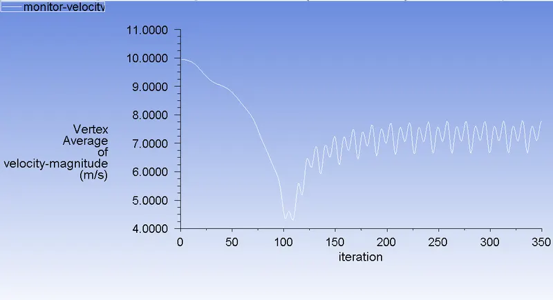
B3) At Re = 1000,

• Material - User defined fluid with rho = 1kg/m^3
• ρ= 1kg/m^3
• μ=0.02 kg/m-s
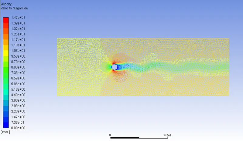
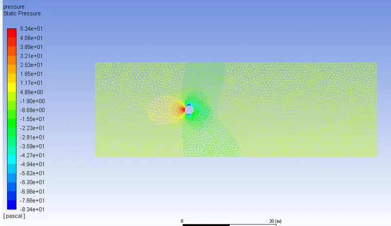
• U = 1000*(0.02/1)/2=>U=10m/s

B4) At Re = 1000,

• Material - User defined fluid with rho = 1kg/m^3
• ρ= 1kg/m^3
• μ=0.02 kg/m-s
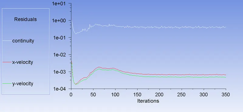
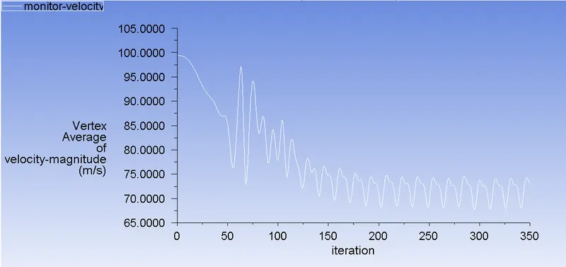
• U = 1000*(0.02/1)/2=>U=100m/s

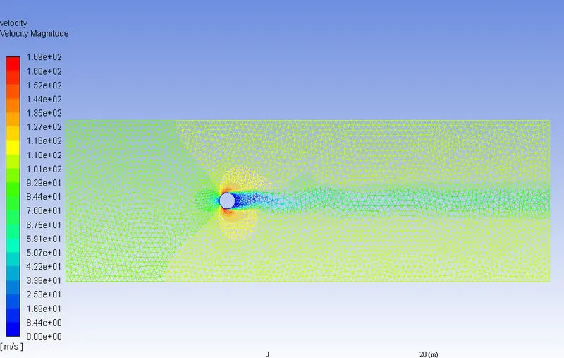
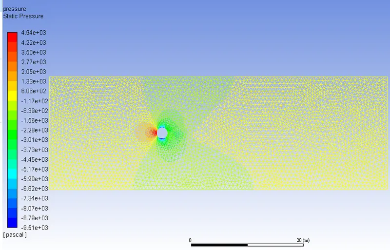
B5) At Re = 100000,

• Material - User defined fluid with rho = 1kg/m^3
• ρ= 1kg/m^3
• μ=0.02 kg/m-s
• U = 10000*(0.02/1)/2=>U=1000m/s

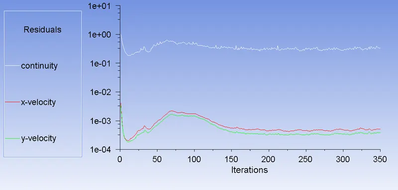
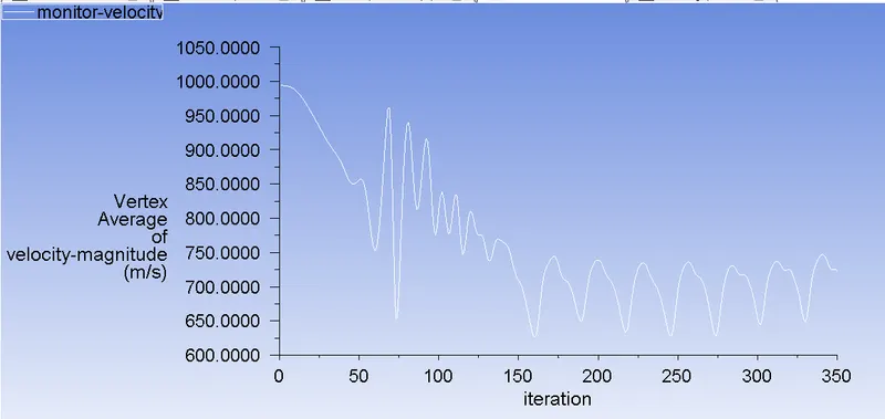
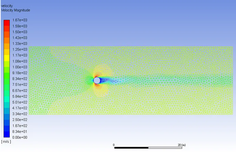
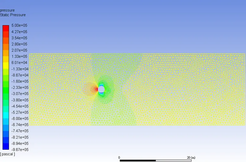
From the above plots and contours, we can see that ass the value of the Reynolds number increased further and further, the wake region is characterized by a pair of counter-rotating vortices that remain attached. At higher Re, as the wake becomes unstable, the viscous forces are no longer sufficient to squash these disturbances. Although the flow is still laminar and 2D, the instability grows further with the increasing Reynolds number,i.e increased levels of turbulence in the boundary layer and wake region.

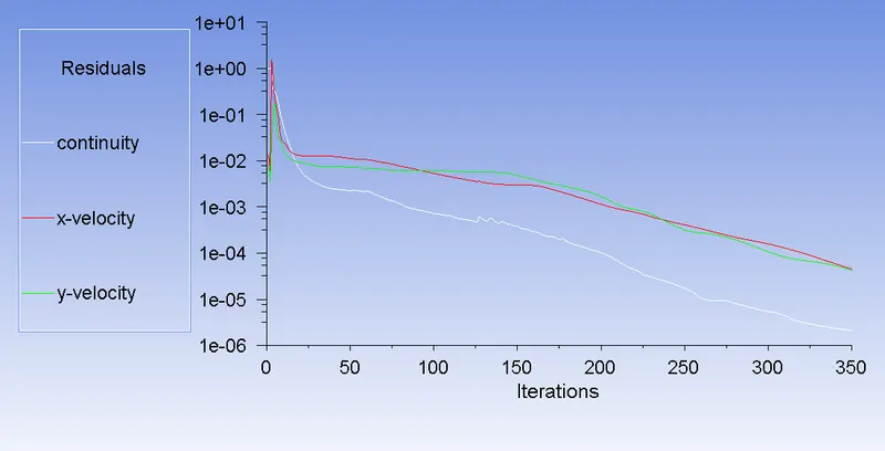
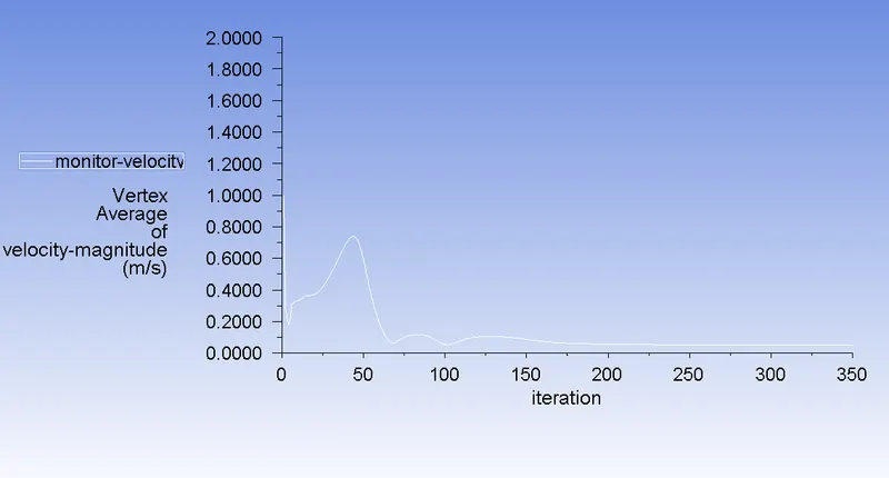
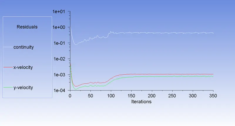
As per our discussion above, in the vortex street simulation, we may probably never get our results fully converged. Thus we need alternate options to see whether our results are converged or not. If we look at the residual plots, we can't determine the solution convergence. But, from the velocity magnitude plots, we can see the repetition of velocity frequency after a certain number of iterations for each run. Which validates our confidence in converged results.

6) phenomenon of Karman vortex street:

n fluid dynamics, a Kármán vortex street (or a von Kármán vortex street) is a repeating pattern of swirling vortices, caused by a process known as vortex shedding, which is responsible for the unsteady separation of flow of a fluid around blunt bodies.

A vortex street will form only at a certain range of flow velocities, specified by a range of Reynolds NUmber(Re), typically above a limiting Re value of about 90. The (global) Reynolds number for a flow is a measure of the ratio of inertial to viscous force in the flow of a fluid around a body or in a channel, and may be defined as a nondimensional parameter of the global speed of the whole fluid flow:

where:

• = the free streamflow speed (i.e. the flow speed far from the fluid boundaries like the body speed relative to the fluid at rest, or an inviscid flow speed, computed through the Bernoulli equation), which is the original global flow parameter, i.e. the target to be non-dimensionalized.
• = a characteristic length parameter of the body or channel
• = the free stream kinematic viscosity parameter of the fluid, which in turn is the ratio:

between:

• = the reference fluid density.
• = the free stream fluid dynamic viscosity.

7) Conclusion -

- The Karman Vortex Street phenomenon for flow over a cylinder is studied and observed in this project.
- Increasing velocity eventually brings the turbulent drag up to and even higher than the laminar drag value, but during the transition from laminar to turbulent, there is a range of Reynolds number, for which turbulent drag is less than laminar drag.
- Vortex shedding can be seen in the case of both steady and transient simulation. But transient simulation produces better and more realistic results.
- Strouhal Number calculation is only possible in the case of transient simulations as the frequency changes concerning time.

Reference :

Links:

https://www.sciencedirect.com/science/article/pii/S0307904X080002 https://www.researchgate.net/publication/312324020_Topological_fluid_mechanics_of_the_formation_of_the_Karman-vortex_street

https://en.wikipedia.org/wiki/K%C3%A1rm%C3%A1n_vortex_street

Books:

Fluid Mechanics Textbook