Week 2 - Flow over a Cylinder.
Objectives:
- To simulate the flow over a cylinder and to explain the phenomenon of vortex karman street.
- to simulate the flow with steady and unsteady flow for the flow with reynold's no of 100 and to calculate the strauhal number for the same.
- to find the coefficient of drag and lift for flow with Reynolds number of 10,100,1000,10000 and 100000
- to discuss the relationship between reynolds number and coefficient of drag.
Introduction:
Vortex karman street effect:
When a fluid such as air or water flows past a bluff body at certain velocities, depending on the size and shape of the body an oscillating flow may take place. This oscillating flow is called as Vortex Shedding.
These vortices are created at the back of the body and detach periodically from either side of the body. These patterns of swirling vortices are repeated periodically and is called as a Von Karman Vortex Street.
Strauhal number:
In dimensional analysis, the Strouhal number is a dimensionless number describing oscillating flow mechanisms.
mathematically its been
St= (FstxD)/U
where
St is strauhal number
Fst is the vortex shedding frequency
D is the dia of cylinder
U is the flow velocity
also with relation to reynolds number it can be given that
St=0.198(1-(19.7/Re))
where Re is reynolds number
Reynolds number:
It is a ratio of dynamic force to Viscous force.
Rn=(dynamic force/ viscous force)= (Density x flow velocity x Diameter)/kinematic viscosity
TASK 1:
- to simulate the flow with steady and unsteady flow for the flow with reynold's no of 100 and to calculate the strauhal number for the same.
mesh:
open space claim geomentry set units to meters
create geomentry similiar to image
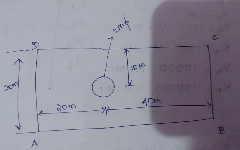
here AD=BC= 20m
CD= AB= 60m
and DIA OF CYLINDER IS 2m
Then go to mesh
name the following edges as as follows
AD = inlet
BC= outlet
AB and CD as symentry
and circle as cylinder
generate mesh with following features
element size 0.25m
no of divisions on circle = 36
inflation layers= 6
growth rate = 1.2
and then generate mesh
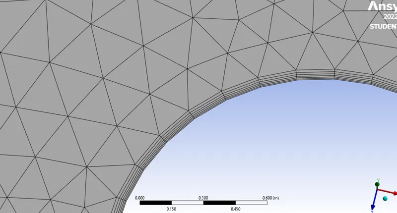
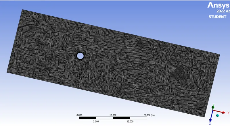
like and thus we completed mesh with these type of mesh we can perform both state of flows with out any errors
mathematical calculation of Strauhal number for Rn of 100
substituting Rn value in eqn
St= 0.198(1-(19.7/Rn))
we get St = 0.16 approx
Steady state:
1. Solver - Steady
2. Type - Pressure Based
3. Viscous Model - Laminar
4. Material - User Material
and for Re of 100 with v= 1m/s and density = 1kg/m3
viscosity = 0.02 Ns/m2
also we need to turn on definition report for
- vertex avg surface report on monitor point at 4D distance from the cylinder
- Contour plots for velocity
set animation to capture shedding
solution method should be simple for 1500 iterations and also there should be hybrid initialization
lets solve the mesh go through reports
scalar residuals
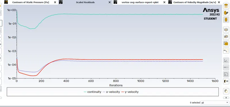
from the graph its visible clearly the solution is converged
velocity contour:
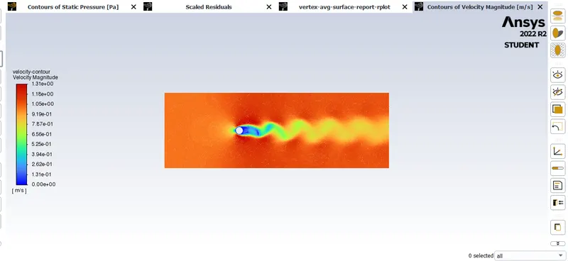
its looks like it is familiar with vortex karman street effect image given initially in this report.
vortex avg at monitor point:
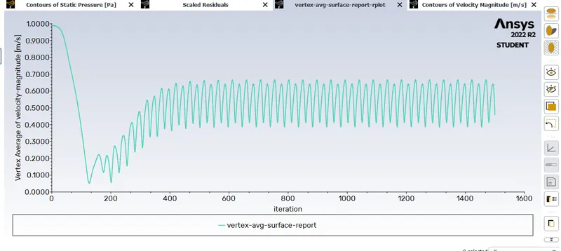
from the above two plots we can easily identify that vortex shedding is accuring in a wave manner
plot for strauhal no at monitor point:
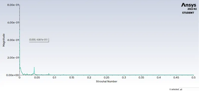
its look difficult so we go for log plot
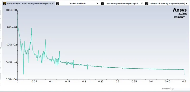
from the graph it is noted that St will be 0.2
most difficult is to identify value such that it is the point where repeated variation starts
UnSteady state:
1. Solver - UnSteady
2. Type - Pressure Based
3. Viscous Model - Laminar
4. Material - User Material
and for Re of 100 with v= 1m/s and density = 1kg/m3
viscosity = 0.02 Ns/m2
also we need to turn on definition report for
- vertex avg surface report on monitor point at 4D distance from the cylinder
- Contour plots for velocity
set animation to capture shedding
solution method should be simple for 0.25 time step iterations and for time steps 1500 and also there should be hybrid initialization
lets solve the mesh go through reports
it will take more time to solve in unsteady case
scalar residuals
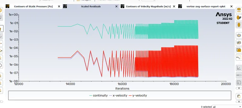
from the graph its visible clearly the solution is converged
velocity contour:
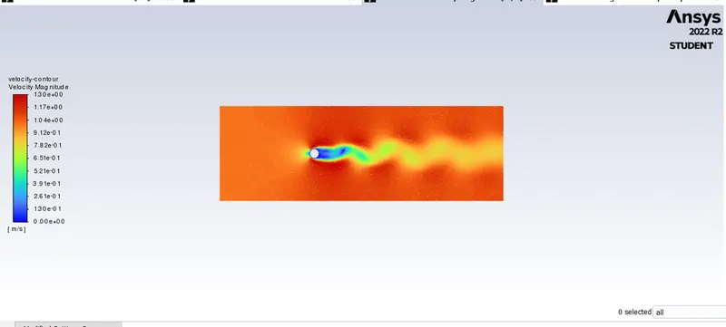
its looks like it is familiar with vortex karman street effect image given initially in this report.
vortex avg at monitor point:
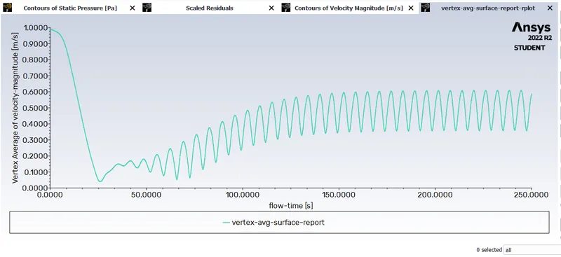
from the above two plots we can easily identify that vortex shedding is accuring in a wave manner
log plot for strauhal no at monitor point:
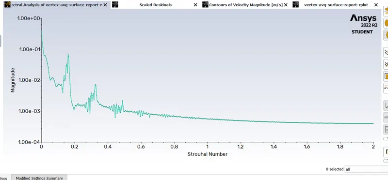
from the graph it is noted that St will be 0.25
most difficult is to identify value such that it is the point where repeated variation starts
while comparing St values on both calculated and analyticals its seems that steady flow produces exact results.
Task 2 : to find the coefficient of drag and lift for flow with Reynolds number of 10,100,1000,10000 and 100000
when substituting values like viscosity; density and diameter in Reynolds number formula it is found to be
Rn= 100 V
hence for
| Rn | Flow Velocity m/s |
| 10 |
0.1 |
| 100 | 1 |
| 1000 | 10 |
| 10000 | 100 |
| 100000 | 1000 |
From table we are going to plot drag coeffeicient and lift in steady state flow (all the values calculated will be approximated)
1.Rn = 10 and v=0.1m/s
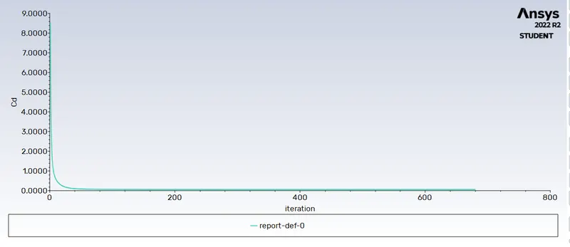
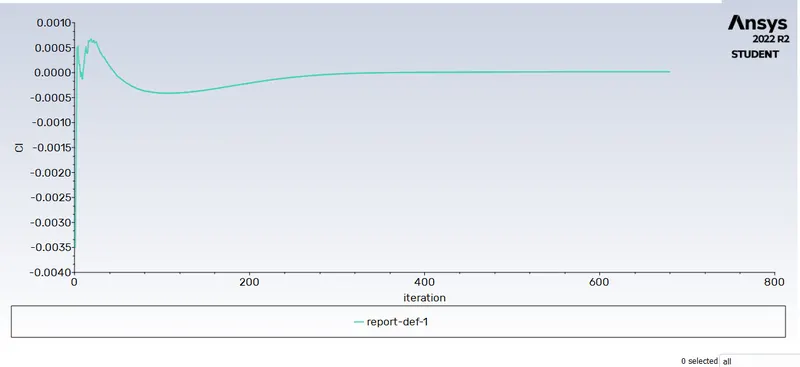
from graph it is found to be coefficient of drag will be 0.1
and coefficient of lift will be more steady after 300 iterations it is found to be 0
so therefore coefficient of lift will be 0.0005 highly
2.Rn=100 and v = 1m/s
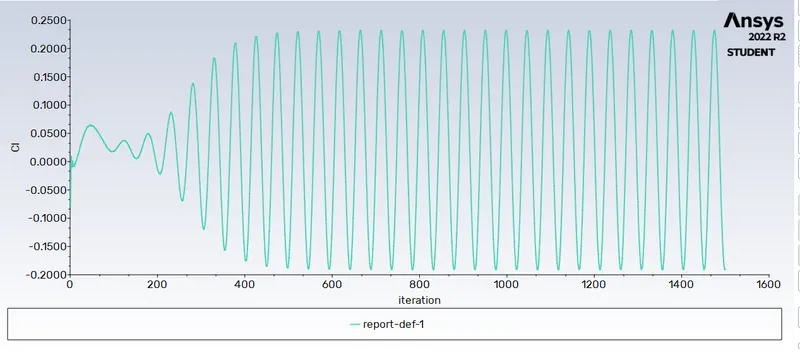
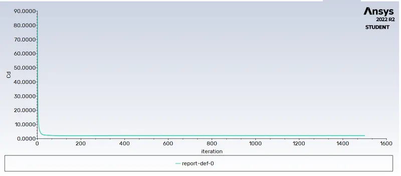
from plots Cd is found to be 4
and then Cl is found to be varying in a range of 0.02
3.Rn=1000 and velocity wil be v=10m/s
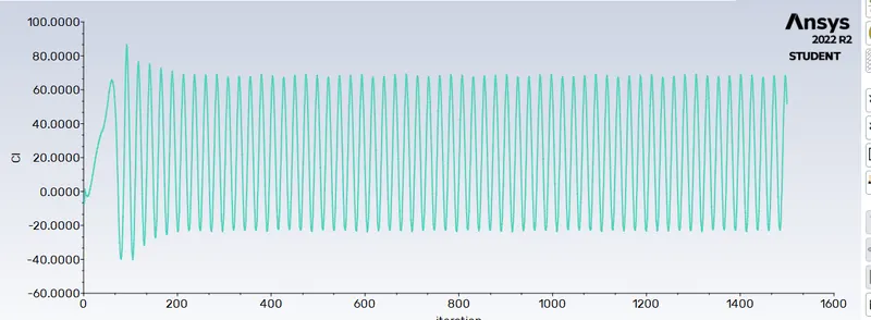
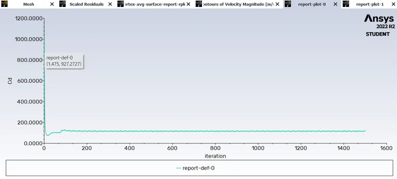
cd is found to be 10
and Cl is found to be 20(which was avg between top and bottom streak)
4.Rn=10000 and v= 100m/s
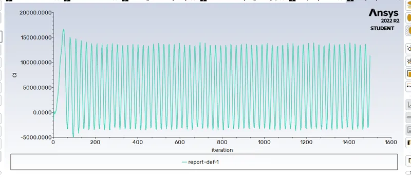
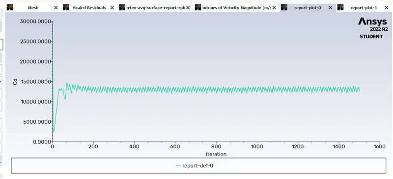
cd is found to be 14000
and Cl is found to be 6000(which was avg between top and bottom streak)
5. Rn= 100000 ; v= 1000m/s
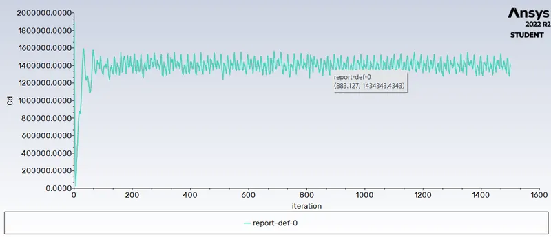
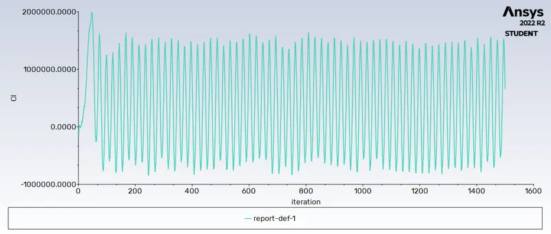
cd is found to be 1400000 and
Cl is 500000
Relationship between Cd and Reynolds number:
When designing a system that will move through a fluid, it is best to measure drag on the system or determine drag through a simulation. It is often helpful to regress the data back to an analytical model. The problem here is that one model does not normally describe all flow behavior in both regimes and the transition region. Instead, the standard practice is to use measured or simulated data to determine models in each flow regime and then examine where these models intersect to determine a transition region.
Laminar Example
The example below is a common model used to relate the drag coefficient vs. Reynolds number for laminar flow across a sphere:
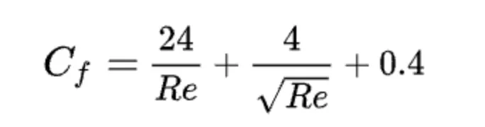
Approximation for drag in laminar flow
This equation is known to be reliable for a broad range of Reynolds numbers in enclosed geometries. An important takeaway is the rough dependence of drag at low Reynolds number (Re < 36), particularly for incompressible or nearly incompressible flows—we find that the drag coefficient is a nearly linear function of velocity. This is the Stokes regime and it is often the starting point for understanding the effects of drag.
Eventually, the above equation will lose its predictive power as the flow transitions into the turbulent regime, and we need a new model to describe the turbulent drag coefficient vs. Reynolds number.
Turbulent Example: Prandlt’s Power Law
Turbulent flow, whether compressible or incompressible, requires a different model that is particular to the type of system being studied. One simple model relating the drag coefficient vs. Reynolds number is Prandlt’s power law. This simple model is defined below:
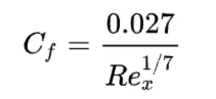
Prandtl’s power law for turbulent flow
In general, the one-seventh power law described above is not applicable to every system, but it is applicable to a wide range of fluids in pipes or other enclosed systems. Drag exerted by turbulence may follow a more complex model with a different power defining the relationship between drag and turbulence. One article in the research literature that contains a review of models relating the drag coefficient vs. Reynolds number can be found below.
also from above calculated values it is found to be as follows
| Rn | Cd |
| 10 |
0.1 |
| 100 | 4 |
| 1000 | 12 |
| 10000 | 14000 |
| 100000 | 140000 |
hence it can be observed for a circular cross section drag coeffeicient increases rapidly with increase in reynolds number
Conclusion:
Thus flow is simulated around circular cross section in steady and unsteady case