Week 2 - Flow over a Cylinder.

Aim:

To simulate the flow over a cylinder and explain the phenomenon of Karman vortex street.

Objective:

PART-I

1. Simulate the flow with the steady and unsteady case and calculate the Strouhal Number for Re= 100.

PART-II

1. Calculate the coefficient of drag and lift over a cylinder by setting the Reynolds number to 10,100,1000,10000 & 100000. (Run with steady solver)
2. Discuss the effect of Reynolds number on the coefficient of drag. [ Results should be validated with any standard literature and error should be within 5 %]

Kármán vortex street

In fluid dynamics, a Kármán vortex street (or a von Kármán vortex street) is a repeating pattern of swirling vortices, caused by a process known as vortex shedding, which is responsible for the unsteady separation of flow of a fluid around blunt bodies.

Experimental measurement shows that the pressure on the rear side (lee side) of the cylinder is less than free stream. Therefore, it follows that the real fluid causes a large pressure-drag force. Besides, the streamlines are not symmetrical with respect to the y-axis. Flow separates from the ream surface and forms a broad, pulsating wake.

Wake consists of pairs of vortices shed alternately from the upper and lower part of the real surface and they are called as Karman Vortex Streets which is s stable configuration for vortex pair. A vortex street can be observed only over a given range of Reynolds numbers (Re), normally above a limiting Re value of about 90. As Re increases, the wake structure becomes more complicated but the alternating shedding can still be detected at Re=10000000. The shedding frequency is defined by the non-dimensionless Strouhal number. Vortex shedding is a viscous flow that evolves into unsteady motions because of flow instability.

Reynolds Number

The transition from laminar to turbulent flow depends on the geometry, surface roughness, flow velocity, surface temperature, and type of fluid, among other things. After exhaustive experiments in the 1880s, Osborne Reynolds discovered that the flow regime depends mainly on the ratio of inertial forces to viscous forces in the fluid. This ratio is called the Reynolds number and is expressed for internal flow in a circular pipe as

Where

V_avg = average flow velocity (m/s),

D = characteristic length of the geometry (diameter in this case, in m),

ρ = density of fluid (kg/m³)

µ = dynamic viscosity (Ns/m²)

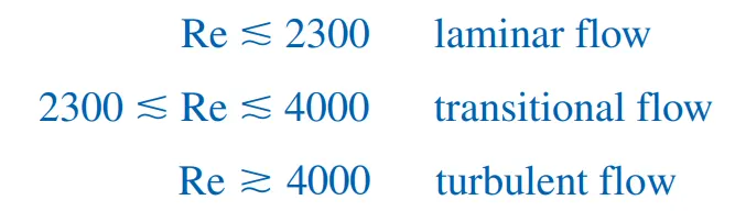
Under most practical conditions, the flow in a circular pipe is laminar for Re ≤ 2300, turbulent for Re ≥ 4000, and transitional in between. That is

Drag & Cofficient of Drag:

The force a flowing fluid exerts on a body in the flow direction is called drag.

Drag is usually an undesirable effect, like friction, and we do our best to minimize it. Reduction of drag is closely associated with the reduction of fuel consumption in automobiles, submarines, and aircraft; improved safety and durability of structures subjected to high winds; and reduction of noise and vibration.

But in some cases drag produces a beneficial effect and we try to maximize it. Friction, for example, is a “life saver” in the brakes of automobiles. Likewise, it is the drag that makes it possible for people to parachute, for pollens to fly to distant locations, and for us all to enjoy the waves of the oceans and the relaxing movements of the leaves of trees

In fluid dynamics, the drag coefficient (commonly denoted as : c_d) is a dimensionless quantity that is used to quantify the drag or resistance of an object in a fluid environment, such as air or water. It is used in the drag equation in which a lower drag coefficient indicates the object will have less aerodynamic or hydrodynamic drag. The drag coefficient is always associated with a particular surface area.

The drag coefficient of any object comprises the effects of the two basic contributors to fluid dynamic drag: skin friction and form drag. The drag coefficient of a lifting airfoil or hydrofoil also includes the effects of lift-induced drag. The drag coefficient of a complete structure such as an aircraft also includes the effects of interference drag.

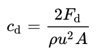
where:

• F_d is the drag force, which is by definition the force component in the direction of the flow velocity
• ρ is the mass density of the fluid;
• u is the flow speed of the object relative to the fluid;
• A is the reference area

Lift & Cofficient of Lift:

A fluid flowing around an object exerts a force on it. Lift is the component of this force that is perpendicular to the oncoming flow direction. Lift conventionally acts in an upward direction in order to counter the force of gravity, but it can act in any direction at right angles to the flow.

In fluid dynamics, the lift coefficient (CL) is a dimensionless quantity that relates the lift generated by a lifting body to the fluid density around the body, the fluid velocity and an associated reference area.

The lift coefficient C_L is defined by

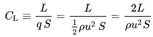
Where L

L is the lift force S

S is the relevant surface area

Q is the fluid dynamic pressure,

ρ is the fluid density

u is the flow speed

STROUHAL NUMBER

The Strouhal Number is a dimensionless value useful for analyzing oscillating unsteady fluid flow dynamics problems.

The Strouhal Number can be expressed as

St = ω l / v

Where

St = Strouhal Number

ω = oscillation frequency

l = characteristic length

v = flow velocity

The Strouhal Number can be important when analyzing unsteady, oscillating flow problems. The Strouhal Number represents a measure of the ratio of the inertial forces due to the unsteadiness of the flow or local acceleration to the inertial forces due to changes in velocity from one point to another in the flow field.

The vortices observed behind a stone in a river, or measured behind the obstruction in a vortex flow meter, illustrates these principles.

STEPS USED FOR SIMULATIONS

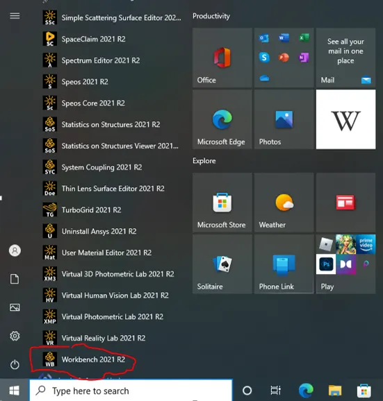
Click on red encircled "Workbench 2021 R2" as shown in the above image to start the simulation.

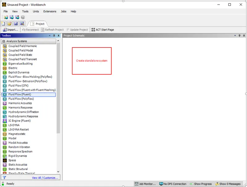
Click On Fluid Flow (Fluent) under Analysis Systems and drag it to create a standalone system.

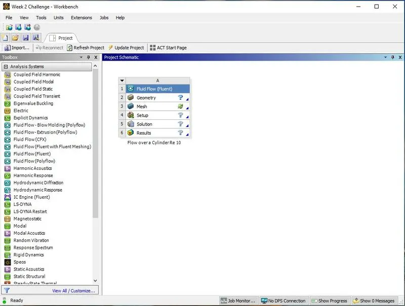
Rename the Project by using the left click and then click the Geometry.

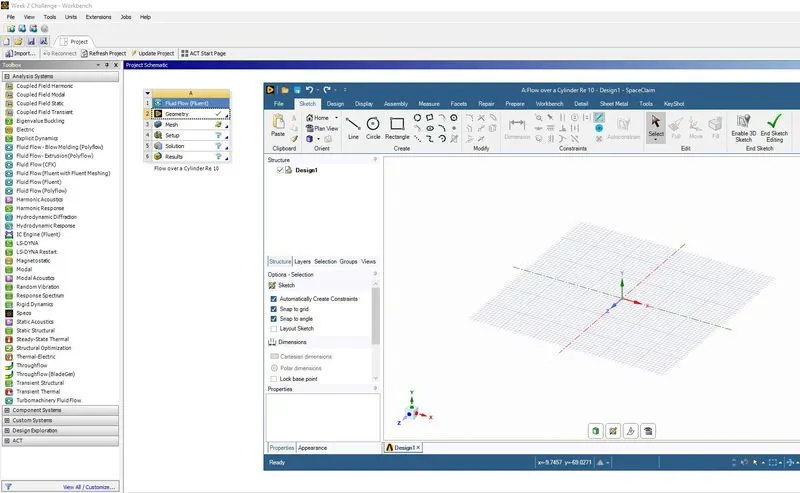
On clicking the geometry, the Space Claim window opens as shown in the above image.

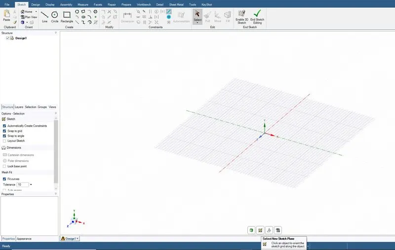
Start the sketching mode and select the sketching plane.

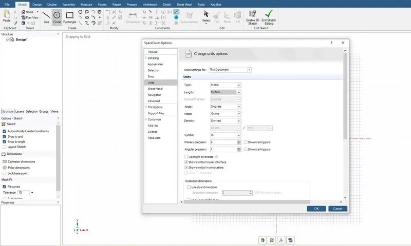
The above option is used to change the unit system.

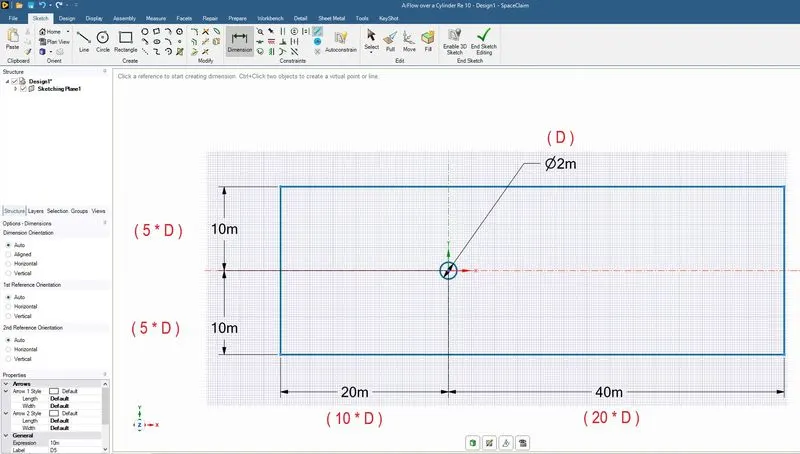
The desired sketch is made using the sketching tools and the parameters shown in the above image.

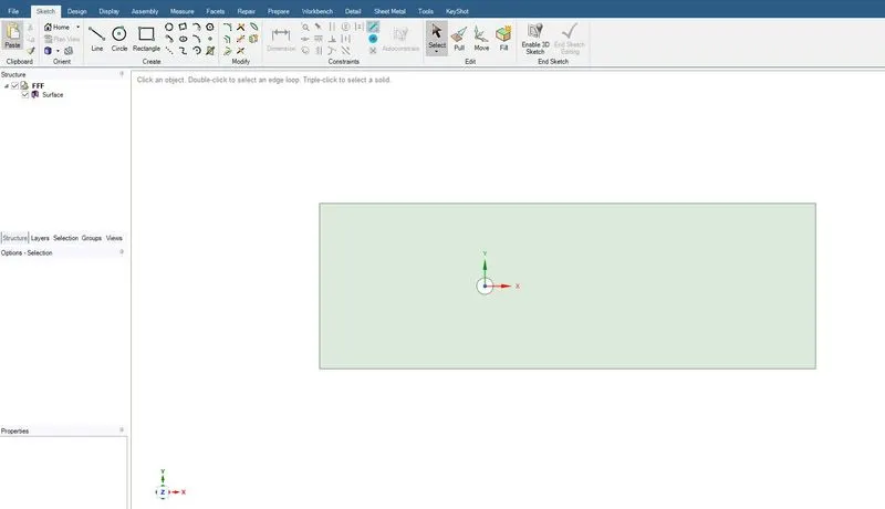
The final geometry passed on to sketching module.

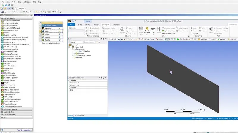
The 2D geometry after opening the meshing module

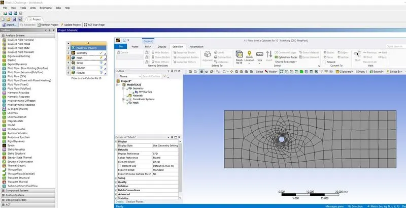
On clicking the Generate Mesh, the tetrahedral mesh is generated as shown in the above image.

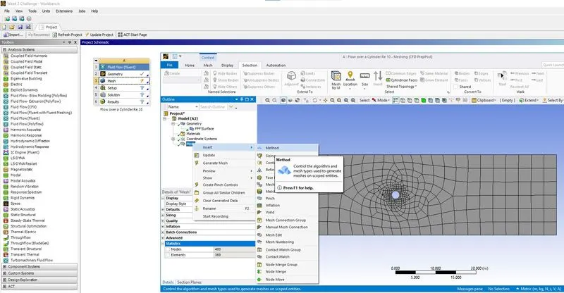
Using Insert Method option as shown in the above image the tetrhedral mesh is changed to triangular.

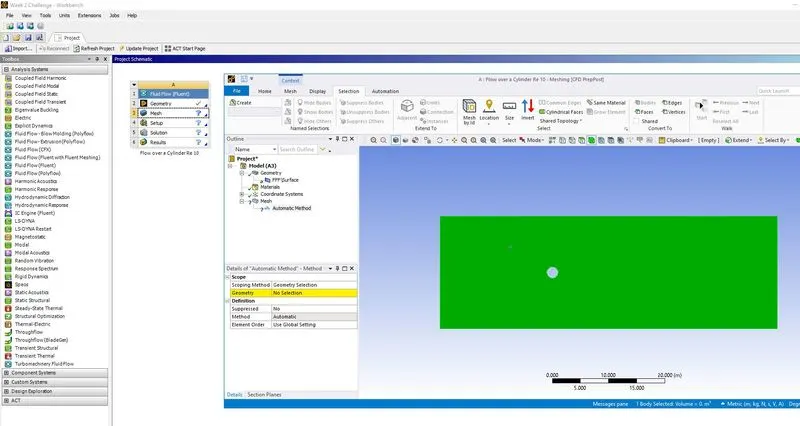
On clicking the Method option a new tab opens on the left hand side where we have select the geometry by clicking on the the yellow highlighted portion and then select the desired geometry where method has to be applied.

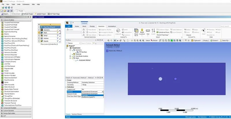
Once the body is selected we change the method from Quadrilateral to Traingles as shown in the above image.

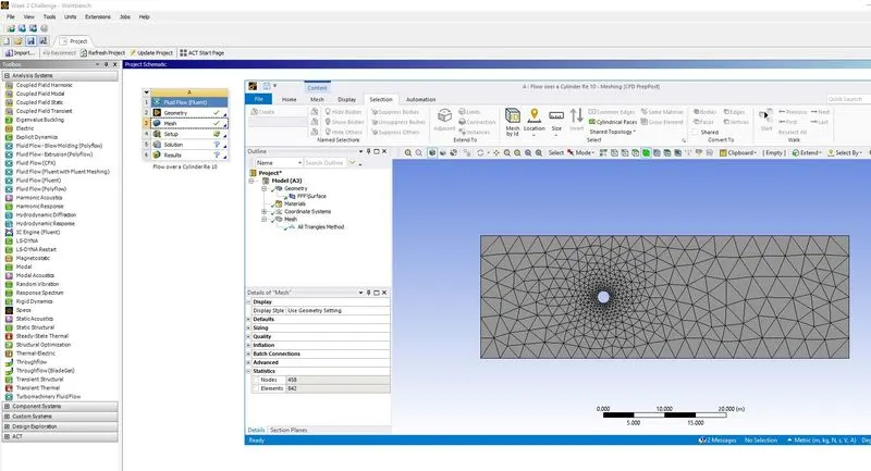
The tetrhedral mesh is converted to traingular mesh.

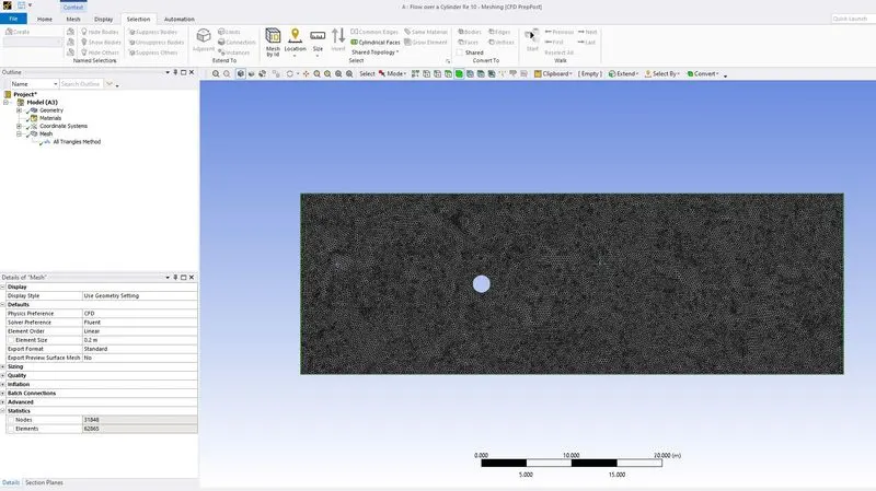
The element size has been changed to 200mm from default value. On updating the Mesh the final ouput is as shown in the above image.

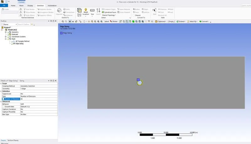
Earlier the shape of the cylinder was looking like a polygon. Using edge sizing we turn the polygon closer to circular shape.

Type used is number of divisions and Number of divisions entered is 36.

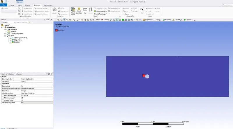
Inflation mesh is an option to use when we need to refine the zone near to the wall. Inflation is use when analysis of boundary condition is done accurately by create finer mesh near to wall or near to boundary. Inflation is also useful for CFD boundary layer resolution, electromagnetic air gap resolution or resolving high stress concentrations.

Now we select the inflation layer. In the Geometry under Scope we select the Face and under definition we select the boundary as edge of circular cylinder.

Under Inflation Option First Layer Thickness is selected and First layer Height is entered 5mm, Maximum layers is considered 20 with a growth rate of 1.2

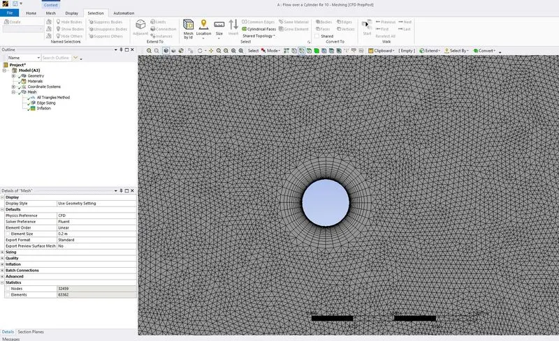
The inflation layer generated near cylinder wall is as shown in the above image.

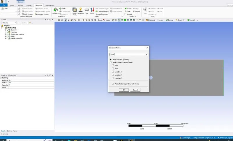
Using Name selection we give the Names to different entity.

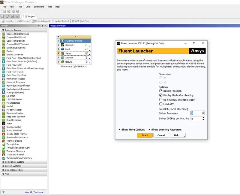
The Ansys fluent set up is launched as shown in the above image.

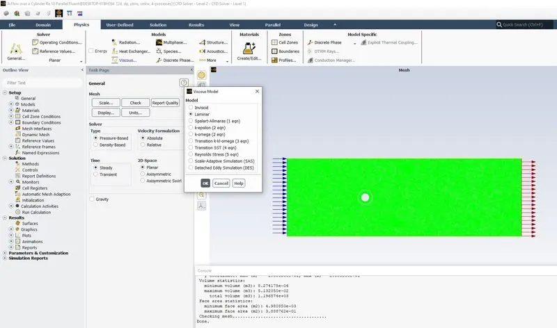
In the viscous model under the Physics>Models the laminar is selected as shown in the above image.

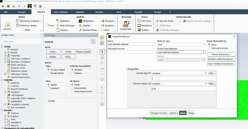
The used defined material for fluis is created with the parameters as shown in the above image.

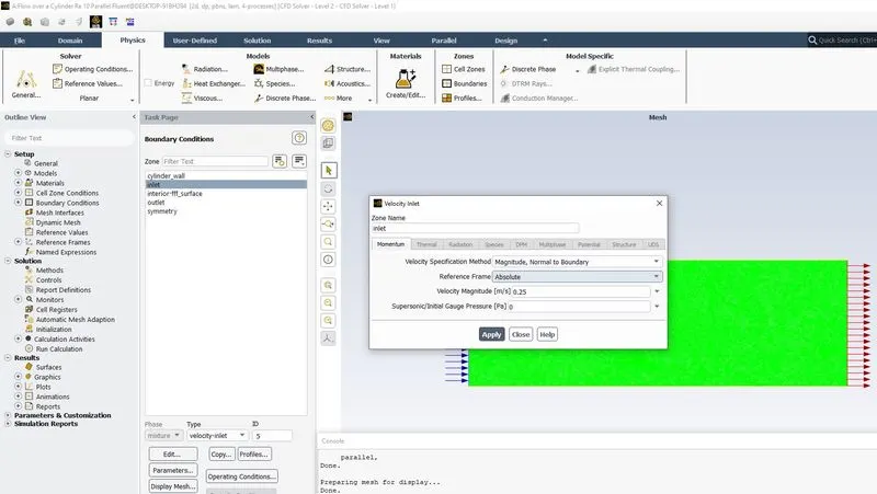
The velocity is entered at the input for the boudary conditions as shown in the above image.

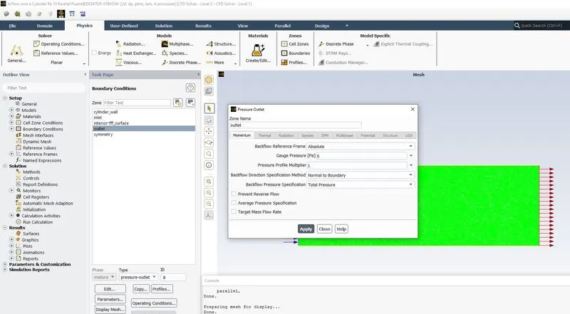
The default pressure is set as the outlet is open to atmosphere as shown in the above image.

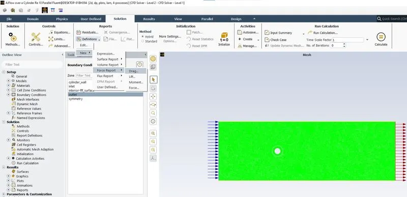
To generate the drag plot the option Solution>Reports>Definitions>New>Force Report>Drag is used as shown in the above image.

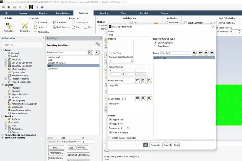
The report is renamed to drag. Under Output Type Drag Coeeficient is selected. cylinder_wall is selected.

Under Create Report File, Report Plot & Print to Console is selected and OK is clicked.

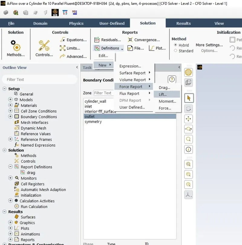
Similar to Drag plot, Lift plot is also defined for plot generation.

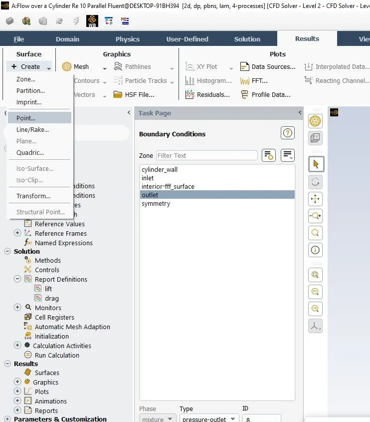
To Create a reference point know as monitor point, Create point in Surface under Results is selected.

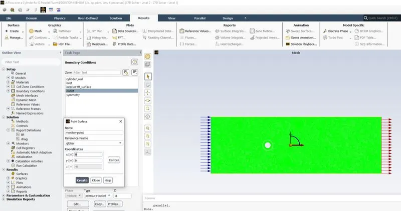
Mointor point location is defined as shown in the above image. Mointor point location is defined as 4 time the Diameter of the cylinder.

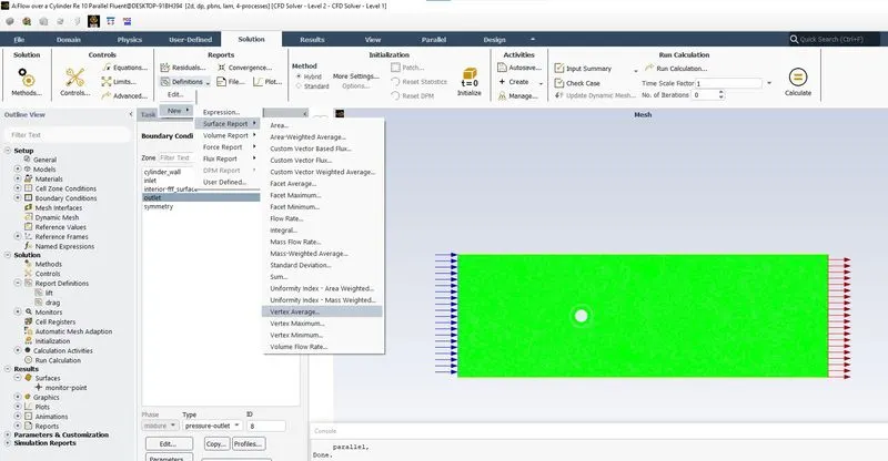
Vertex average velocity at mointor point is defined as shown in the above image.

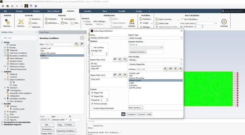
The similar steps are followed for plot generation definition.

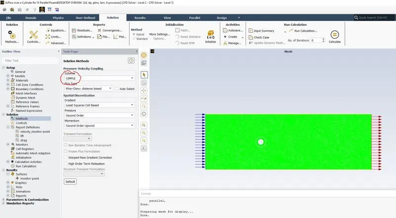
Under the Solution Methods, the Pressure Velocity Coupling Scheme is changed to SIMPLE from the default (i.e. Coupled)

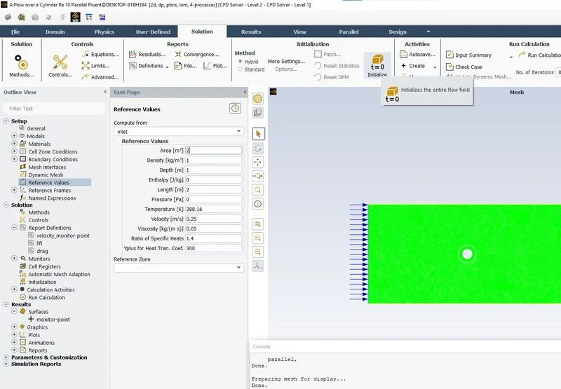
In Reference Values under Setup, Compute from In let is selected by drag down. Length is changed to 2 and Area is changed to 2.

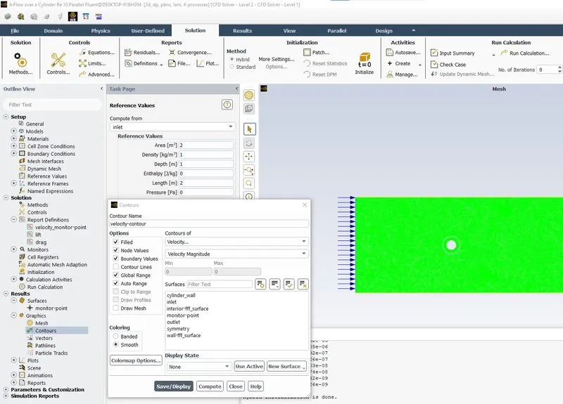
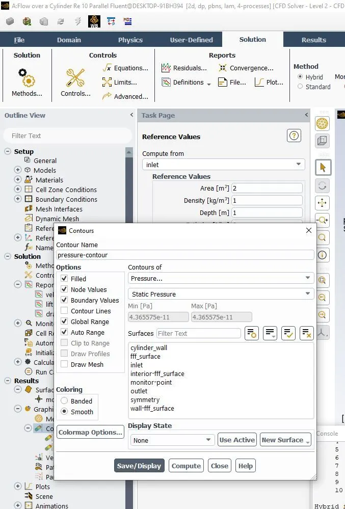
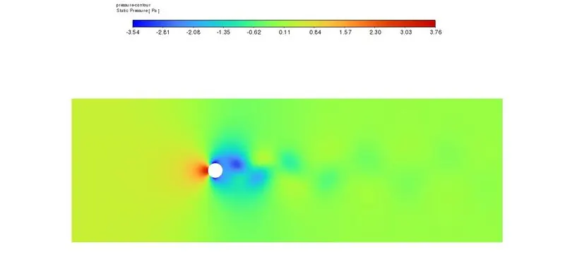
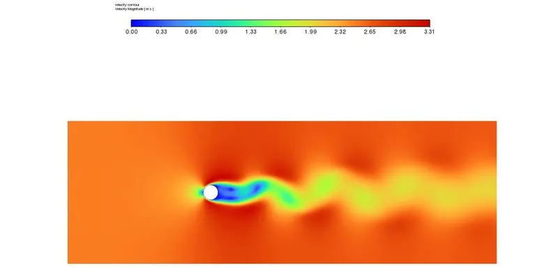
After changing the reference values, Initialization is done. After Initialization, the Pressure conoturs and velocity contours are defined as shown in the below two images.

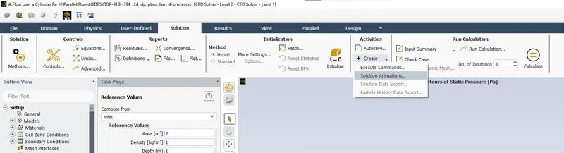
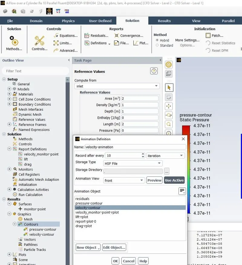
To create the solution animation, the option shown in the above image gets activated

Procedure to calculate Strouhal Number in Ansys Fluent

• Open Fluent
• Click on plots under Results
• Then select FFT plot
• After that, load the input file (Lift or velocity plot)
• Then, change the X axis to Strouhal number and Y axis to Magnitude
• After that, click on Plot FFT
• Once the plot is generated Write FFT option is enabled. Click on write FFT
• Then, open the FFT file using excel or notepad and then, find out the stouhal number value for maximum magnitude (Maximum Peak)

The following cases done using ANSYS Fluent(Refer the below Image)

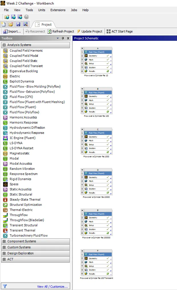
1) REYNOLD'S NUMBER Re = 100 (Transient/ Unsteady State)

1.1 DRAG PLOT

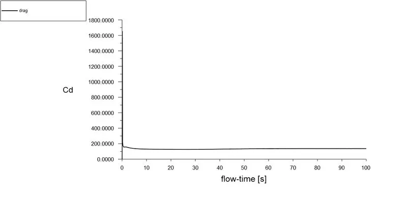
Here the coeeficient of drag converges after 20 seconds

1.2 LIFT PLOT

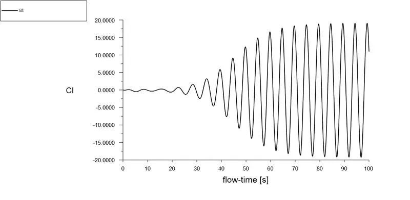
Here the coefficient of lift converges after 70 seconds

1.3 STROUHAL NUMBER VS MAGNITUDE PLOT

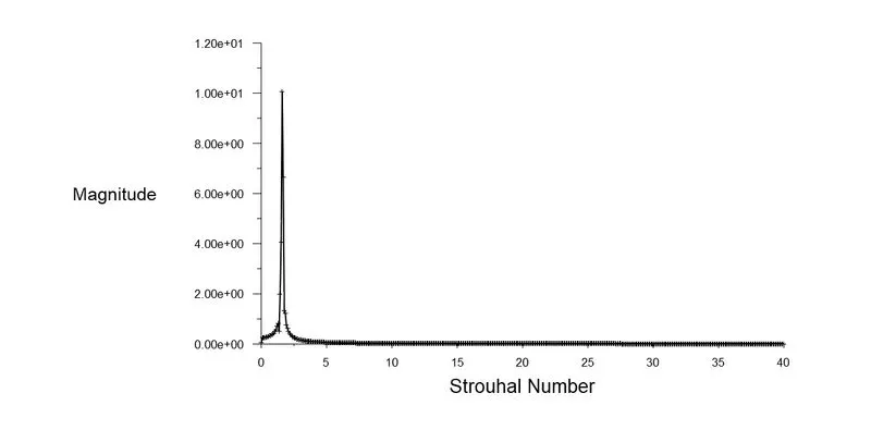
The Strouhal number is 0.0096

1.4 SCALED RESIDUALS

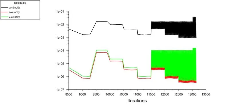
Here the scaled residuals converges after 11500 iterations.

1.5 VERTEX AVERAGE OF VELOCITY MAGNITUDE AT MONITOR POINT

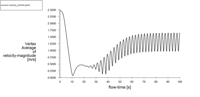
Here the vertex average of velocity magnitude at monitor point converges in between 70 - 80 seconds.

1.6 PRESSURE CONTOUR

1.7 VELOCITY CONTOUR

1.8 ANIMATION

https://drive.google.com/file/d/1uu8JEE0r2PyRtBOba0DiRE66mGI-KeF8/view?usp=sharing

2) REYNOLD'S NUMBER Re = 100 (Steady State)

2.1 DRAG PLOT

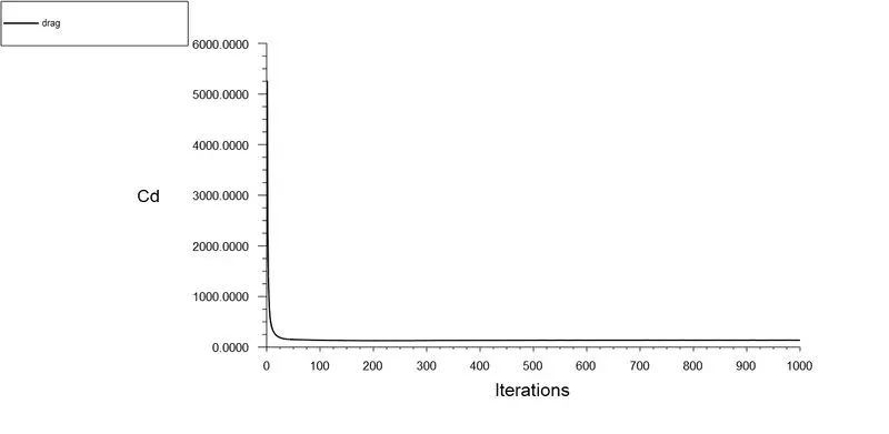
Here the coefficient of drag converges after 50 iterations.

2.2 LIFT PLOT

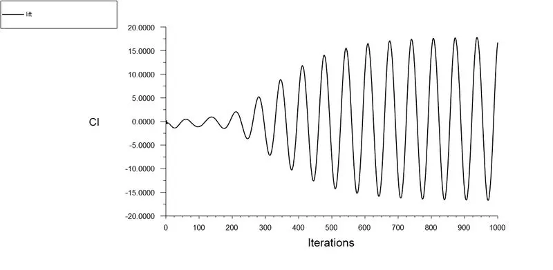
Here the coefficient of lift converges after 700 iterations.

2.3 STROUHAL NUMBER VS MAGNITUDE PLOT

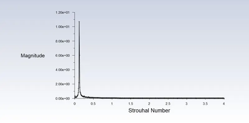
The Strouhal number is 0.008

2.4 SCALED RESIDUALS

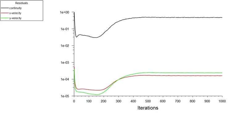
Here the scaled residuals converges after 500 iterations.

2.5 VERTEX AVERAGE OF VELOCITY MAGNITUDE AT MONITOR POINT

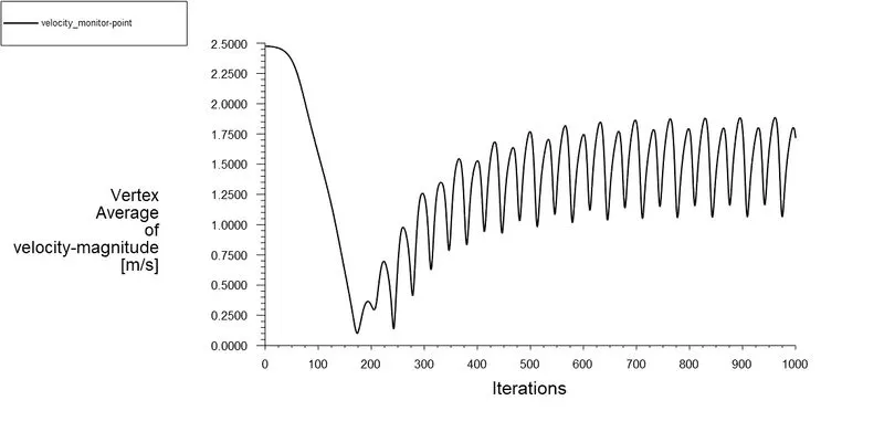
Here the vertex average of velocity magnitude at monitor point converges after 600 iterations

2.6 PRESSURE CONTOUR

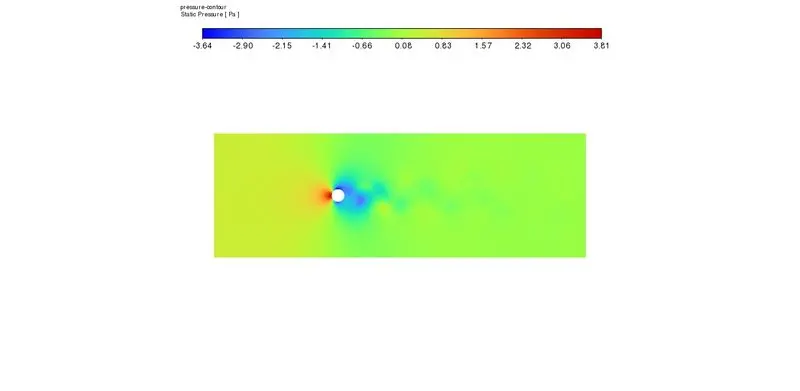
2.7 VELOCITY CONTOUR

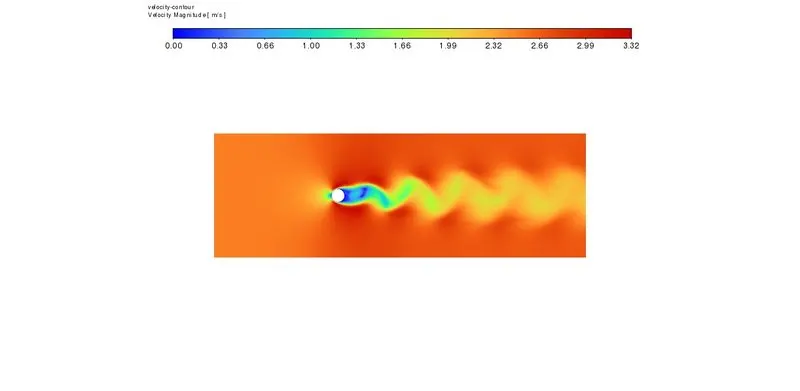
2.8 ANIMATION

https://drive.google.com/file/d/14DoevGVxXrYL75hpUrCIwDZrSH9vNFNd/view?usp=sharing

3) REYNOLD'S NUMBER Re = 10 (Steady State)

3.1 DRAG PLOT

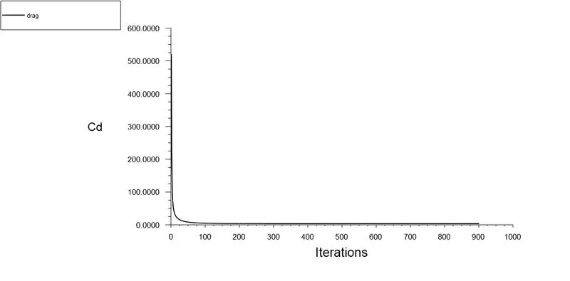
Here the coefficient of drag converges after 100 iterations.

3.2 LIFT PLOT

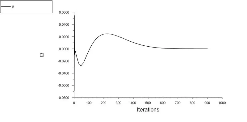
Here the coefficient of lift converges after 700 iterations.

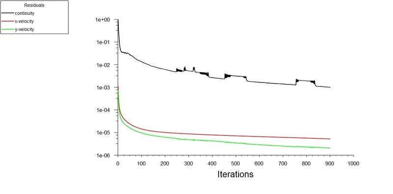
3.3 SCALED RESIDUALS

3.4 VERTEX AVERAGE OF VELOCITY MAGNITUDE AT MONITOR POINT

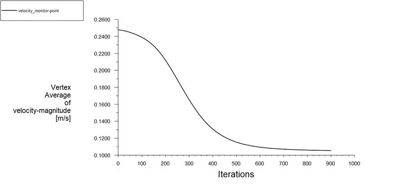
Here the vertex average of velocity magnitude at monitor point converges after 800 iterations

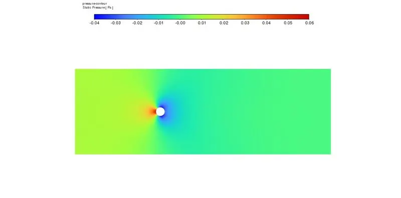
3.5 PRESSURE CONTOUR

3.6 VELOCITY CONTOUR

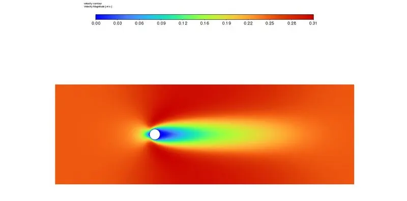
4) REYNOLD'S NUMBER Re = 1000 (Steady State)

4.1 DRAG PLOT

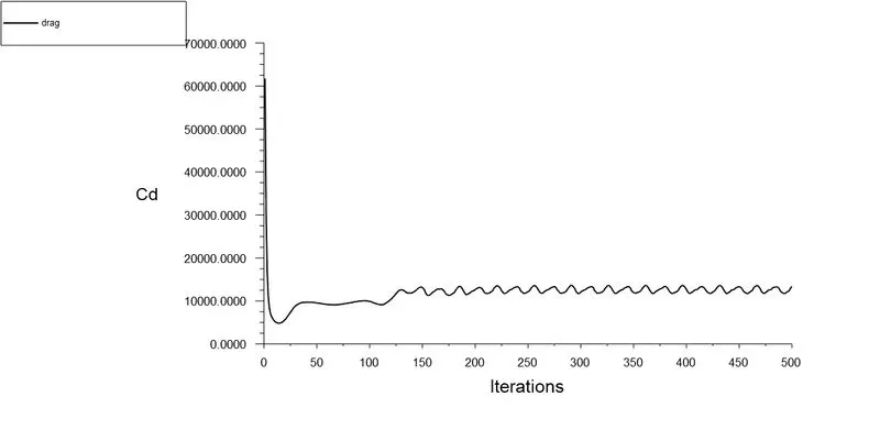
4.2 LIFT PLOT

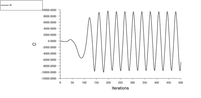
4.3 SCALED RESIDUALS

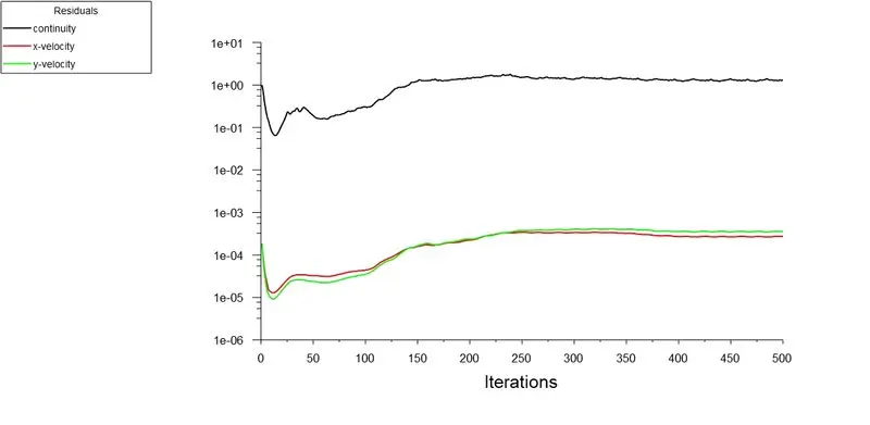
4.4 VERTEX AVERAGE OF VELOCITY MAGNITUDE AT MONITOR POINT

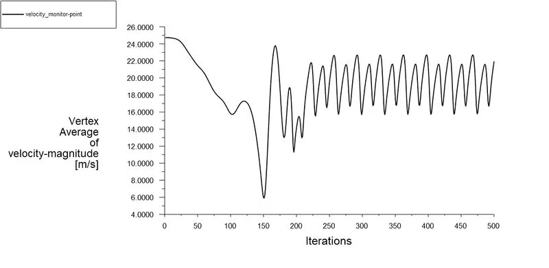
Here the vertex average of velocity magnitude at monitor point converges after 250 iterations

4.5 PRESSURE CONTOUR

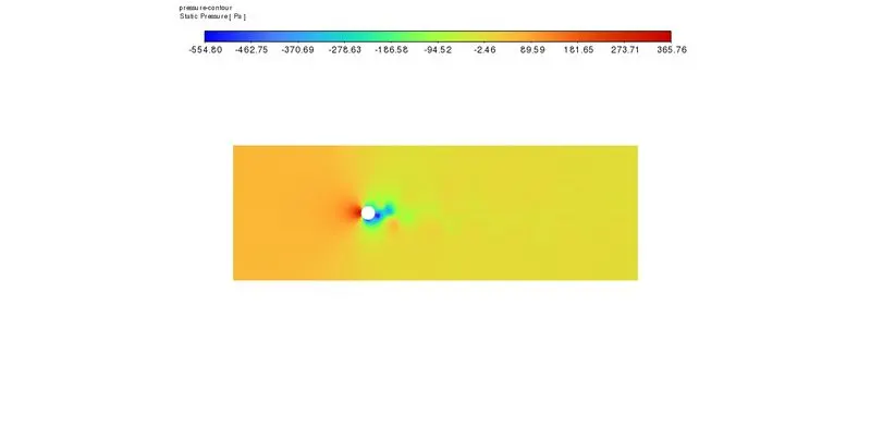
4.6 VELOCITY CONTOUR

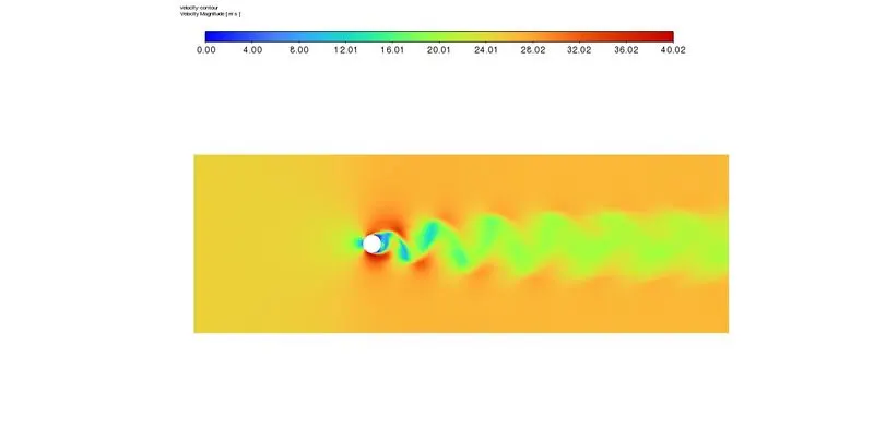
5) REYNOLD'S NUMBER Re = 10000 (Steady State)

5.1 DRAG PLOT

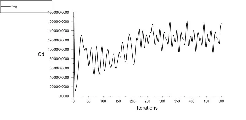
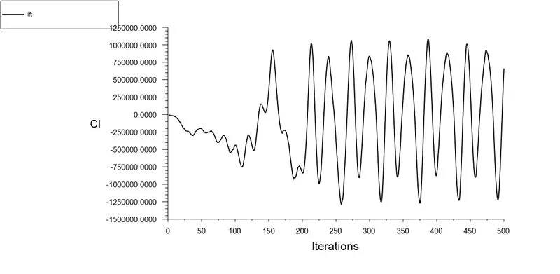
5.2 LIFT PLOT

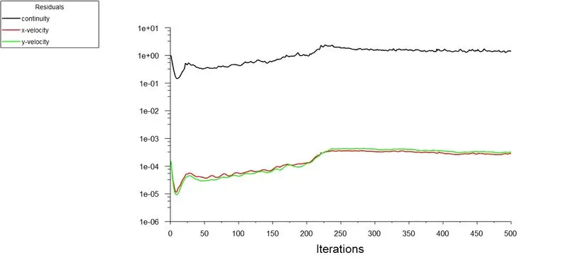
5.3 SCALED RESIDUALS

5.4 VERTEX AVERAGE OF VELOCITY MAGNITUDE AT MONITOR POINT

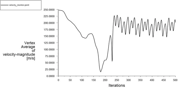
Here the vertex average of velocity magnitude at monitor point converges after 300 iterations

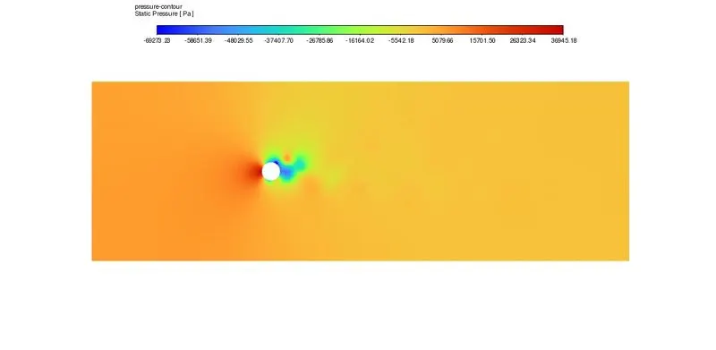
5.5 PRESSURE CONTOUR

5.6 VELOCITY CONTOUR

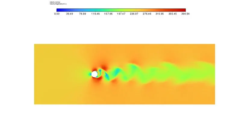
6) REYNOLD'S NUMBER Re = 100000 (Steady State)

6.1 DRAG PLOT

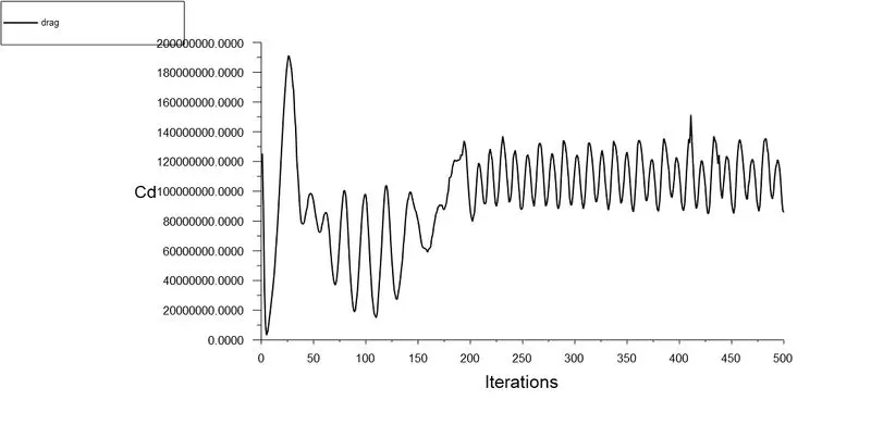
6.2 LIFT PLOT

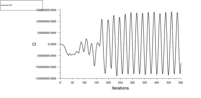
6.3 SCALED RESIDUALS

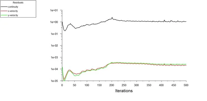
6.4 VERTEX AVERAGE OF VELOCITY MAGNITUDE AT MONITOR POINT

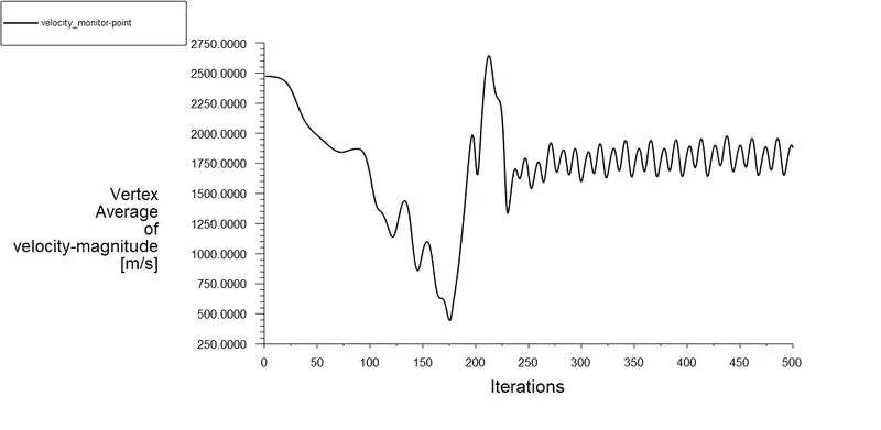
Here the vertex average of velocity magnitude at monitor point converges after 300 iterations

6.5 PRESSURE CONTOUR

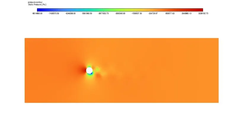
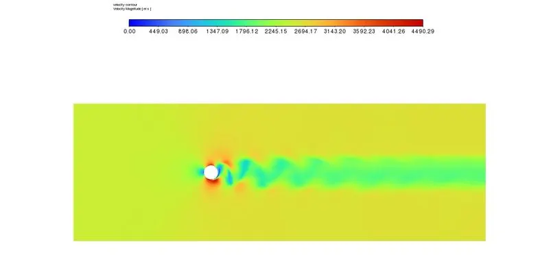
6.6 VELOCITY CONTOUR

SUMMARY

For Steady State & Transient State Simulations the Coefficient of Drag and Coeeficient of Lift are tabulated as follows:

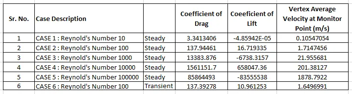
Table 1

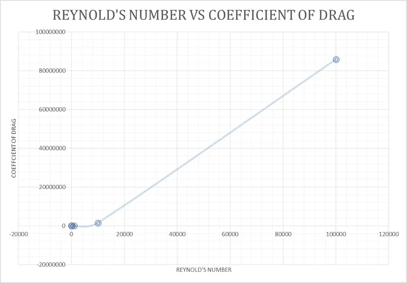
PLOT 1

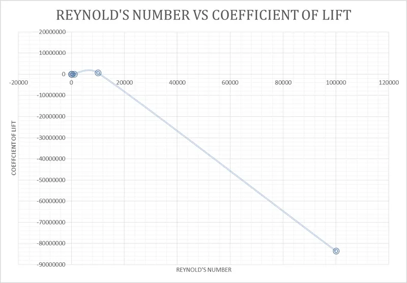
PLOT 2

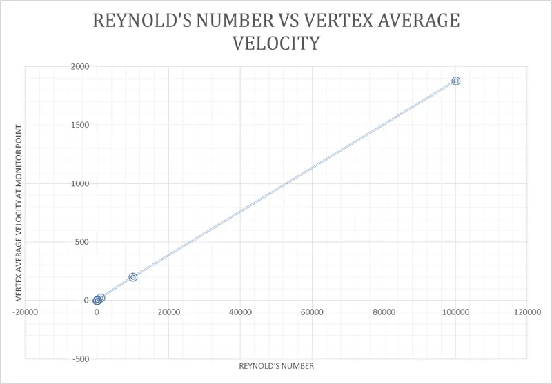
PLOT 3

CONCLUSION:

• From PLOT 1 (Reynold's Number vs Coefficient of Drag), we conclude that the coefficient of drag increases with an increase in reynold's number.
• From PLOT 2 (Reynold's Number vs Coeeficient of Lift), we conclude that the coefficient of lift varies with varying frequency with an increase in reynold's number.
• From PLOT 3 (Reynold's Number vs Vertex Average Velocity At Monitor Point), we conclude that the velocity increases with an increase in monitor point
• From velocity contours we can arrive at a conclusion that there is an increase in wake region behind the cylinder with an increase in reynold's number.
• Vortex shedding takes place only after the reynold's number 100 and above.

REFERENCES:

WIKIPEDIA

NASA WEBSITE

FLUID MECHANICS BY YUNUS CENEGAL

SCIENCE DIRECT