Week 2 - Flow over a Cylinder.

Aim: Simulating a flow over a cylinder and study the affects of flow parameters on the simulation results.

The challenge at hand is divided into 2 challenges:

1. For Reynolds NumberRe=100, simulate the flow using steady and unsteady/transient solver independently and compare the results.
2. Using a steady solver solve simulate the flow over the cylinder with varying Reynolds Number.

Theory: When a blunt body is placed in flow field the flow is seperated from considerable portion of the body. i.e: the flow will not be in contact for the entire length of body along the flow direction. Over a certain value of Renynolds number (Re), the flow in the wake region is characterised by formation of unsteady vortices in alternating pattern. Such a phenomenon is called Kármán vortex street.

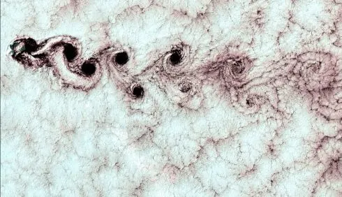
The Karman Effect is also visible on a symmetrical body like - a cylinder, which is very non-intuitive as we presume that a laminar uniform flow over a symmetric body should give a symmetric flow in the wake region. But, such is not the case. The phenomenon shall be verified through simulation and the reasons shall be made clear in the conclusion section of this challenge.

Simulation Setup:

1. Case Setup:
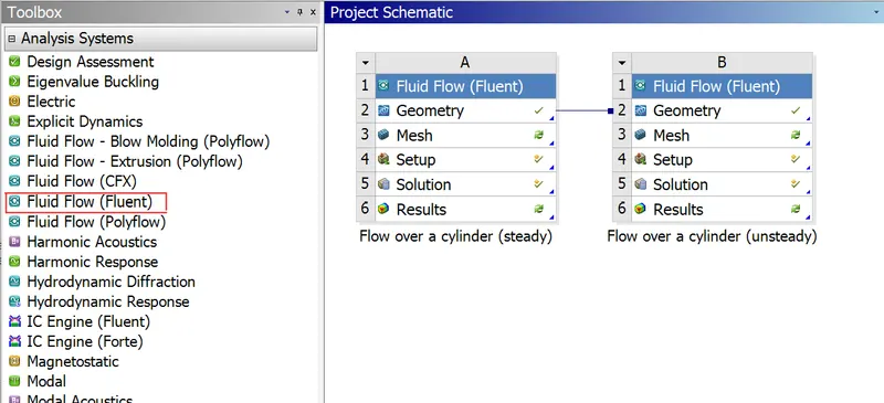
   Since we are using same geometry for steady and unsteady cases we can link the geometry for both case setups
   
   
2. Geometry Setup:
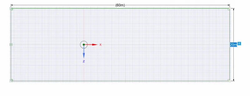
   We have considered a domain of size 60 m x 20 m and a cylinder body of diameter 2m placed at 20m from the left face. The geometry is made in space claim and is in 2D form as we are going to assume the flow dosent vary in the direction perpendicular to the plane.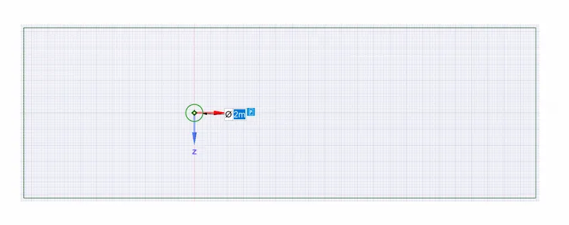
   
3. Meshing:
   A proper meshing is crucial for obtaining results which agrees to experimental data and physical intuition. If meshing is not done properly, then solution might converge but will not be consistent with the experimental data.
   We will be using a triangular mesh.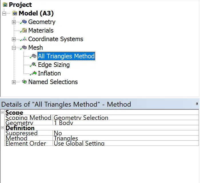
   
   
   
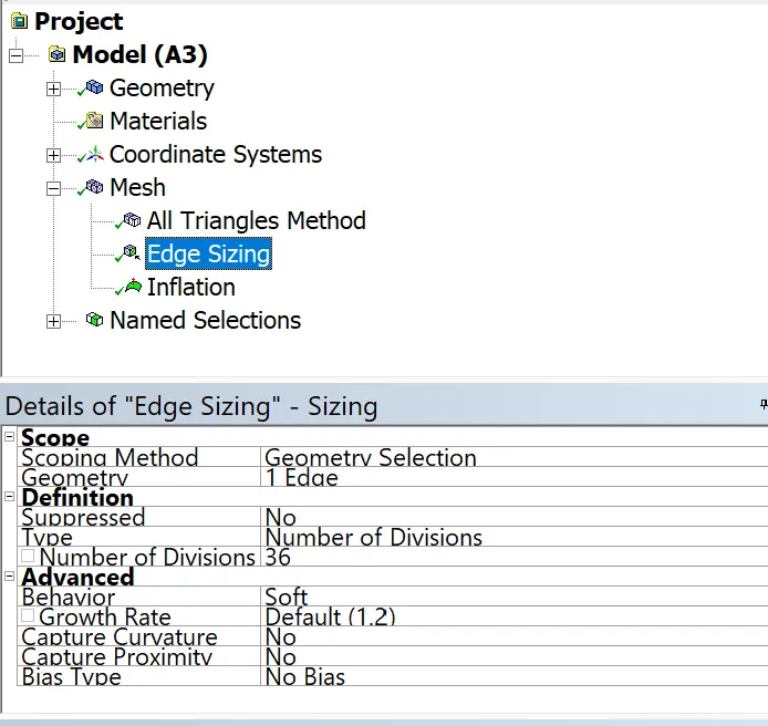
   Since the wall of the body is circular and the mesh generated are not that smooth- it looks more like a polygon than a circle. In order to smoothen out the edges, we opt for edge sizing control as shown above.
   For capturing the boundary layer effects we add inflation layers near the walls.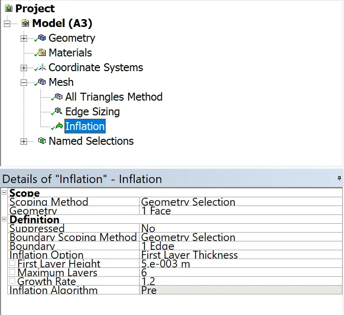
   
   
   
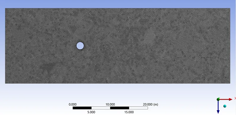
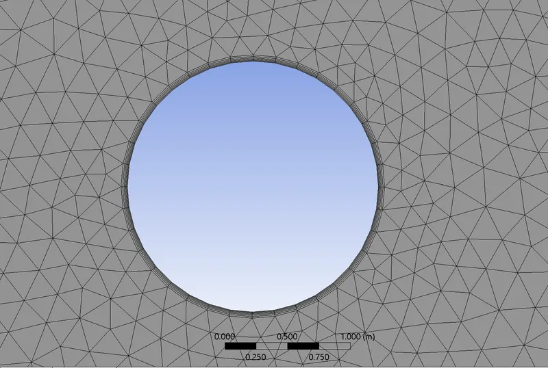
   final mesh inflation layers in mesh
   
   
4. Setup:
   The setups differ for Steady and Unsteady cases. For Steady Case we have a steady state and pressure based solver assuming the flow is incompressible.
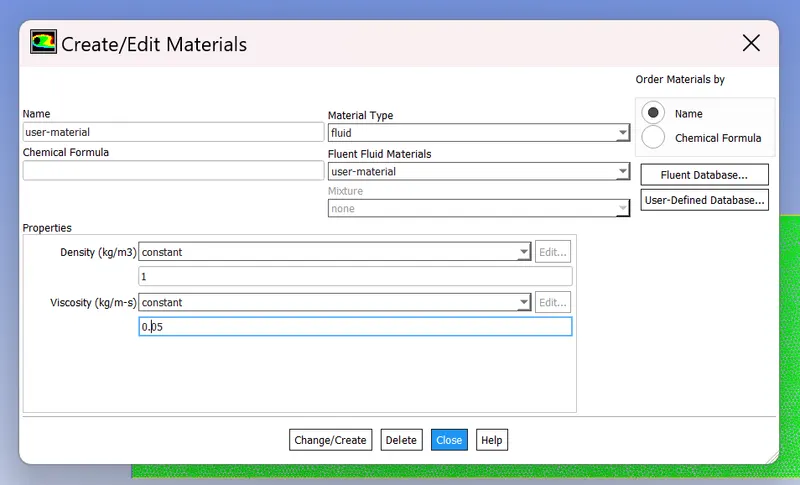
   The material is defined with values chosen and modified in such a way so as to meet the Reynolds number requirement.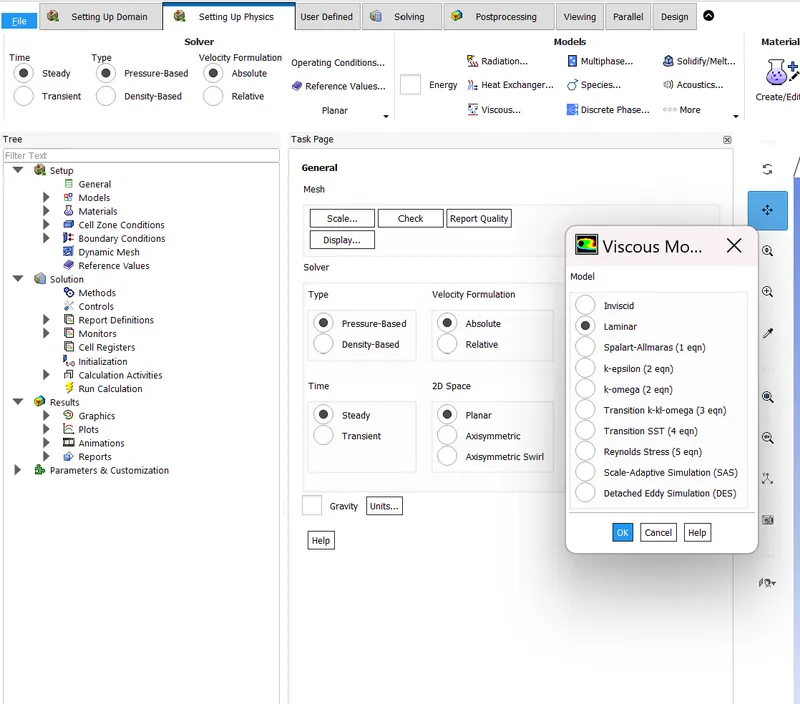
   
   
   
   
   A monitor point is created.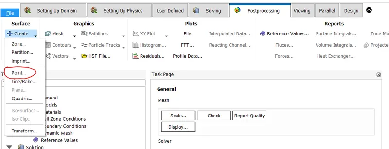
   
   
   
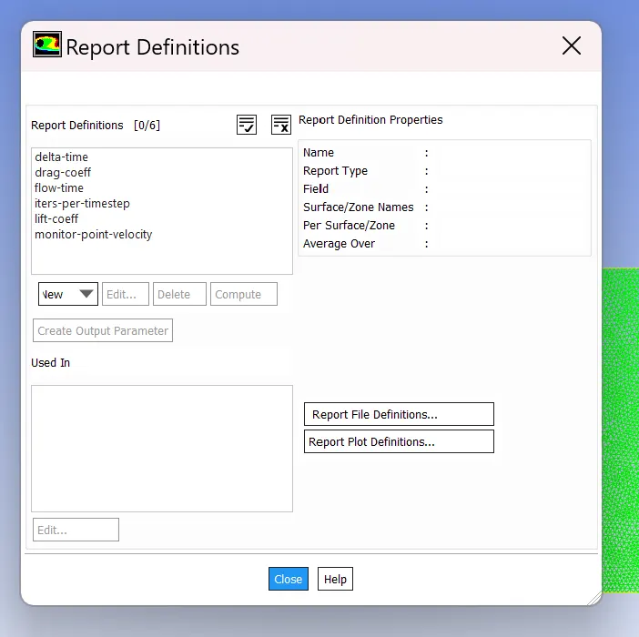
   Report Definitions are defined for simulation results. Also reference values should be appropriately defined else Cd and Cl values obtained will be inconsistent with the actual results.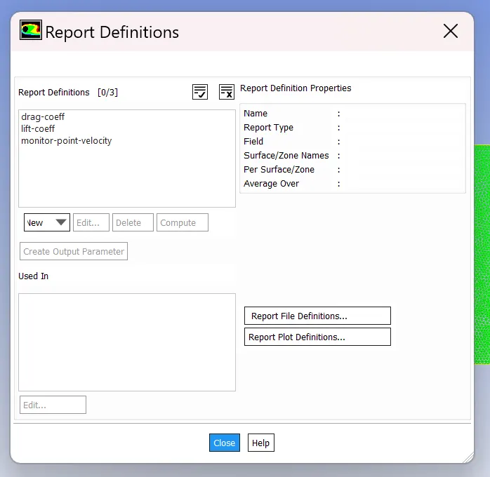
   
   
   
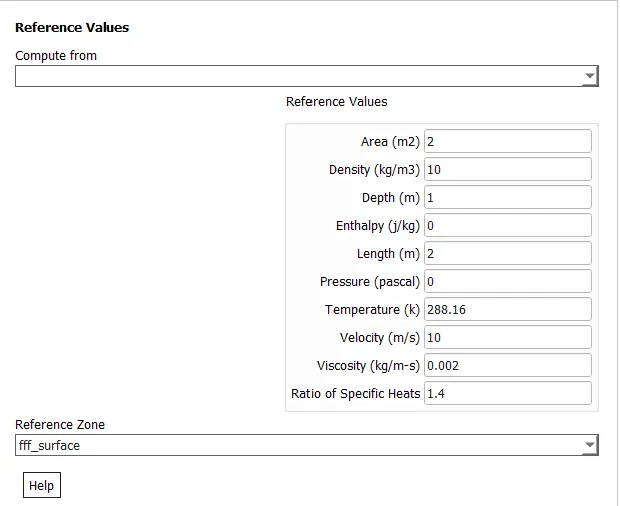
   The simulation is initialized and is runned for a provided number of iterations. The results of each iteration is visible and updated in console window and also on graphics window.
   
   For Unsteady Case however things are different. The solver is transient solver which leads to ansys asking for another input as time step value.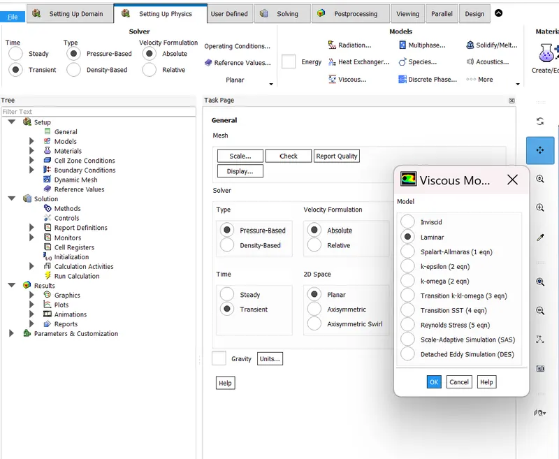
   
   
   
   
   
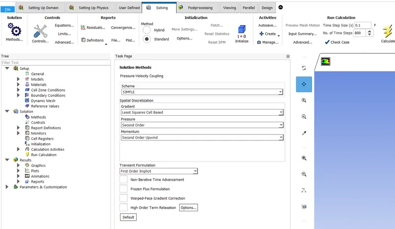
   Since time domain is also included we can check for strouhal number for unsteadiness of the flow.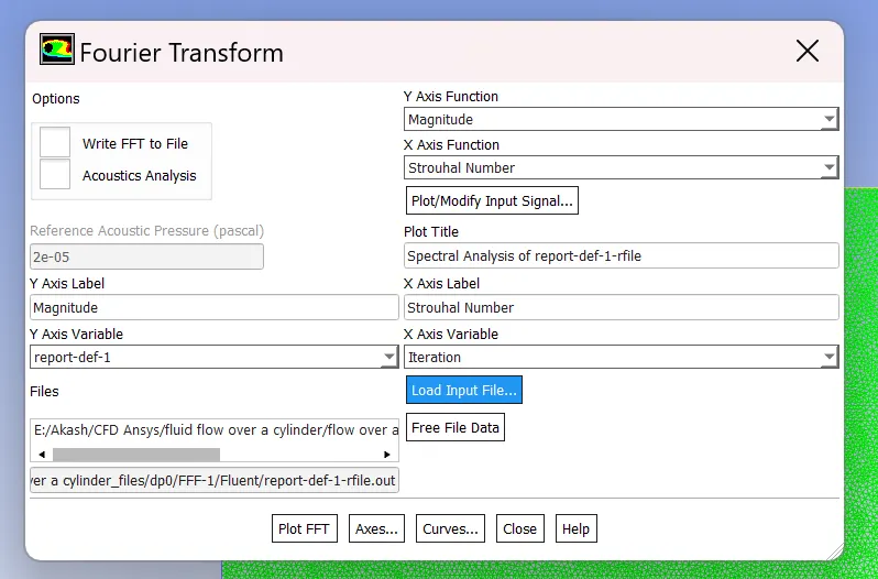
   
   
   
   
5. Results:
   
   Case 1: Steady Case vs Unsteady Case at Re=100
   
   Following plots were obtained-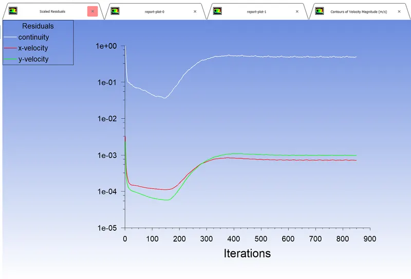
   
   
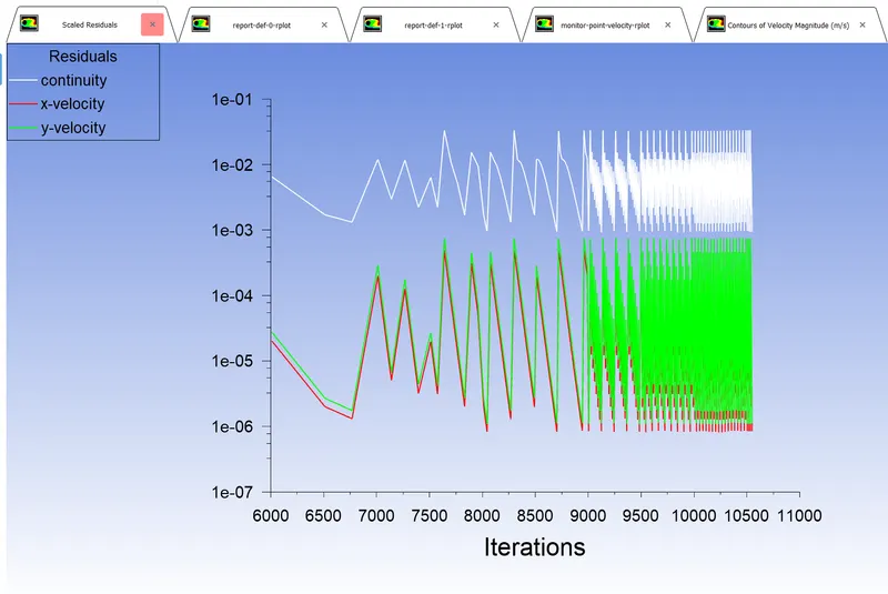
   scaled residue steady case scaled residue unsteady case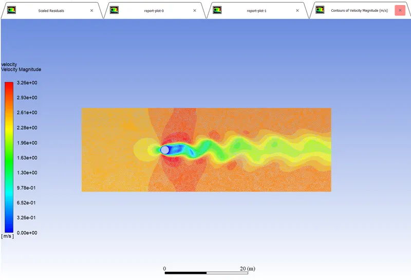
   
   
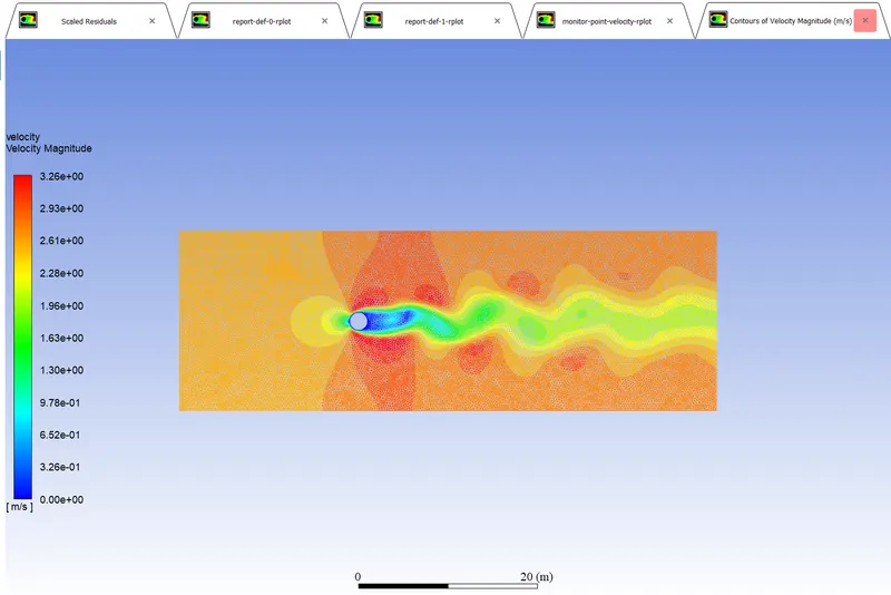
   velocity contour plot (steady) velocity contour plot (unsteady)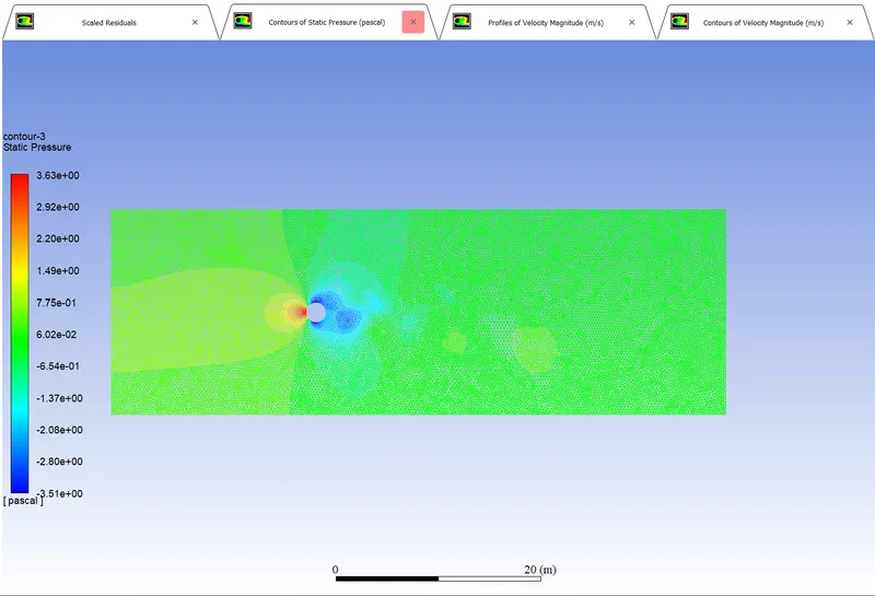
   
   
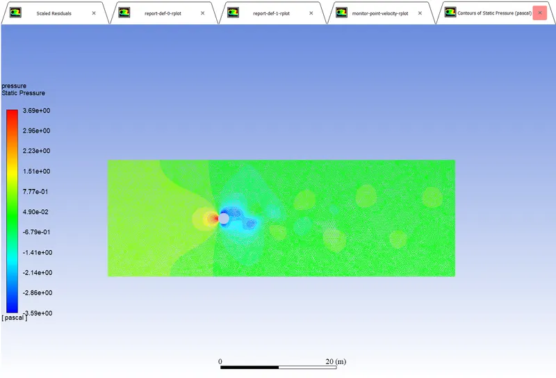
   pressure contour plot (steady) pressure contour plot (unsteady)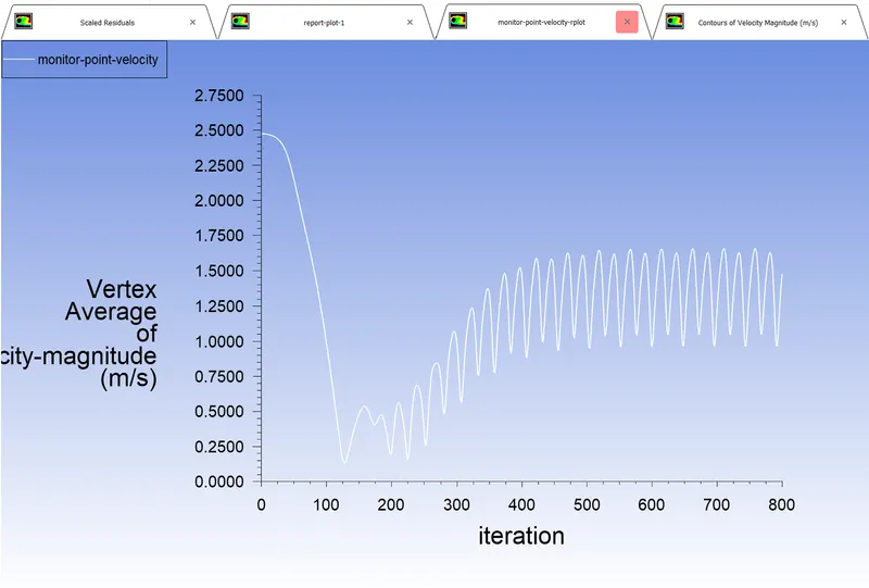
   
   
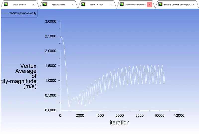
   velocity at monitor point (steady) velocity at monitor point (unsteady)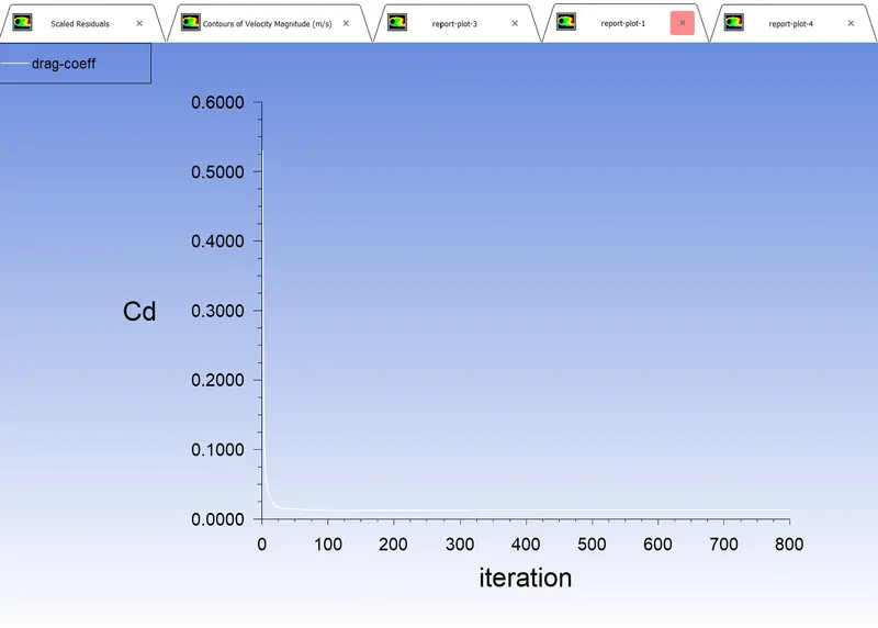
   
   
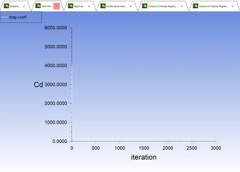
   coefficient of drag (steady) coefficient of drag (unsteady)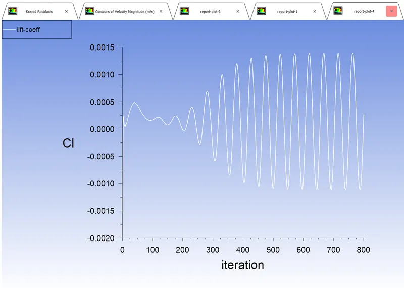
   
   
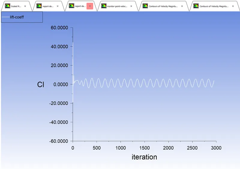
   coefficientt of lift (steady) coefficient of lift (unsteady)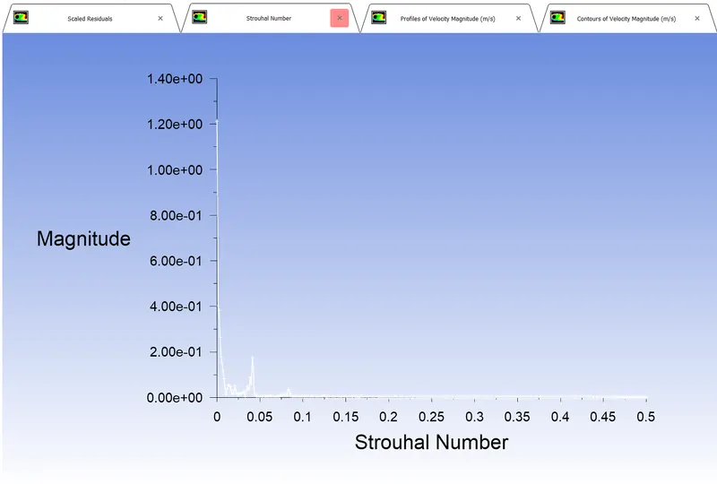
   
   
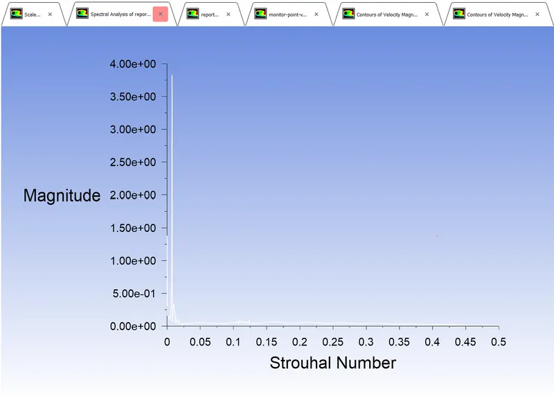
   Strouhal number plot (steady) Strouhal number plot (unsteady)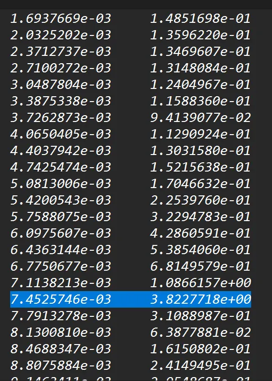
   
   
   strouhal number (unsteady)
   
   Case 2: Coefficient of Drag and Coefficcient of Lift for Re=10, 100, 1000, 10000, 100000
   
   Following Results were obtained-
   
   

   Reynolds Number (Re)	Coefficient of Drag (Cd)	Coefficient of Lift (Cf)
   10	0.033244	8.16e-06
   100	0.013365	0.0002641
   1000	0.717112	0.1562491
   10000	0.780662	0.7589521
   100000	0.953177	0.0919154

   
   
   
6. Conclusions:
   
   General-
   As the fluid flows over the cyinder it seperates from the body after travelling a certain distance over the body in the direction of the flow. However until certain Reynolds Number is achieved the flow doesn't show alternate vortex shedding. it just joins again downstream and is uniform again. As seen in low Re flow of 10.
   
   However as Re increases alternate vortex shedding is visible. This also implies that "Symmetric geometry doesn't guarantee symmetric flow". The reason is that due to presence of small non uniformity is flow field variables. These non uniformities gets amplified in wake region with increasing Re, consequently increasing the unsteadiness of the flow as well. This aspect of the flow is captured using Strouhal Number (St).
   `St=f_(st)D/V`where `f_(st)`is frequency of oscillations of vortex shedding, D is the characteristic length (in our case diameter of the cylinder)
   
   Case 1-
   
   From our Case 1 Results, we have obtained vortex shedding in steady and unsteady cases. But the Strouhal Number obtained for Steady solver doesnt have any significance as in steady iterations doesn't account for time variables and each of the peak and the trough values of velocity doesn't correspond to any particular time step. Hence, we don't have any record of time step or frequency which makes Strouhal number meaningless in steady case. However, in case of unsteady case it is very relevant and is obtained as a result from the simulation results.
   The Strohal number gives the idea about the unsteadiness of the flow. Higher the number implies more the frequency of the oscillations of vortex shedding and moe is the unsteadiness of the flow. For our case Strouhal Number (St) came out to be equal to 0.0074.
   
   Case 2-
   
   For Steady cases, as Re value increases Cd and Cl values increases as evident from the tabular data achieved from the simulations.
   Higher values of Cd implies the wake region is broadening and boundary layer is transitioning from laminar to turbulent.
   Higher values of Cl refers to high pressure difference between top and bottom of the body hinting again that the flow is transitioning towards turbulency.
   
   
7. References-
   https://www.cfd-online.com/
   Flow around a Circular Cylinder -Fluid Mechanics by Yunus A. Cengel, John M. Cimbala, Pg 897.