Week 2 - Flow over a Cylinder.
Aim :
To Simulate the flow over a cylinder and explain the phenomenon of Karman vortex street.
Objectives :
PART-I
- Simulate the flow with the steady and unsteady case and calculate the Strouhal Number for Re= 100.
PART-II
- Calculate the coefficient of drag and lift over a cylinder by setting the Reynolds number to 10,100,1000,10000 & 100000. (Run with steady solver)
- Discuss the effect of Reynolds number on the coefficient of drag. [ Results should be validated with any standard literature and error should be within 5 %]
Expected results:-
- In both approaches, show that the flow has converged. That is, what quantities or plots need to be looked at to determine that the flow has converged?
- Plots of the coefficient of drag and lift.
- Plots to show vortex shedding behind the cylinder.
- Mention the referred material (Reference Paper or Fluid Mechanics Textbook) at the end of the challenge submission page.
1. Flow over cylinder:
- In spite of extensive experimental and numerical studies almost over a century, flow around a circular cylinder still remains a challenging problem in fluid mechanics, where intensive investigations are continued even today to understand the complex unsteady dynamics of the cylinder wake flow.
- Cross-flow normal to the axis of a stationary circular cylinder and the associated problems of heat and mass transport are encountered in awide variety of engineering applications. Both experimental measurements and numerical computations have confirmed the onset of instability of the wake flow behind a cylinder beyond a critical Reynolds number, leading finally to a kind of periodic flow identified by definite frequencies, well-known in the literature as the Von Karman vortex street.
- In case of laminar flow past cylinders with regular polygonal cross-section, the flowusually separates at one or more sharp corners of the cross-section geometry itself, forming a system of vortices in the wake on either side of the mid symmetry plane.
- On the other hand, for a circular cylinder, where the point of flow separation is decided by the nature of the upstream boundary layer, the physics of the flow is much more complex than what its relatively simple shape might suggest.
This report emphasis on the analysis of two-dimensional flow over a circular cylinder in different Reynolds number. The analytical solution of the same case modeled with the potential flow is known and easy to interpret; however, the physical mechanism which rules real flow around a circular cylinder, as well as its mathematical treatment, is highly complex. Some examples are the boundary layer detachment and oscillatory effects that without a CFD study would be very difficult to determine either analytically or experimentally.
The unconfined or free flow past a circular cylinder exhibits a rich variety of flow regimes depending upon the intrinsic nature of the flow. It needs to be emphasized here that at finite Reynolds number, two flow regimes can be identified in the vicinity of the cylinder, i.e., the boundary layer of thickness, which is usually much smaller than the diameter of the cylinder and the wake region which is of the order of one-to-two times the diameter. Notwithstanding the fundamental significance of delineating the conditions for the transition from one flow regime to another, this information is also germane to develop the scaling laws for the gross engineering parameters like drag and lift coefficients, Strouhal number, and Nusselt number with the Reynolds number and Prandtl number. Therefore, significant research effort has been expended on exploring this aspect in this field. It is thus instructive to recapitulate the key points pertaining to the onset and distinguishing features of various flow regimes documented for the uniform transverse flow of Newtonian fluids past an unconfined smooth circular cylinder which is long in the transverse direction thereby eliminating the complications arising from the surface roughness and end effects, respectively.
For the aforementioned simple flow, the flow is governed by the familiar Reynolds number.
ReL=ULvo">`ReL=ULvoReL=ULvo`
Where,
U = the free stream flow speed.
L = a characteristic length parameter of the body or channel
vo">vovo = the free stream kinematic viscosity parameter of the fluid
vo=μoρ0">`vo=μoρ0vo=μoρ0`
ρ">ρρ = fluid density
μo">μoμo = dynamic viscosity
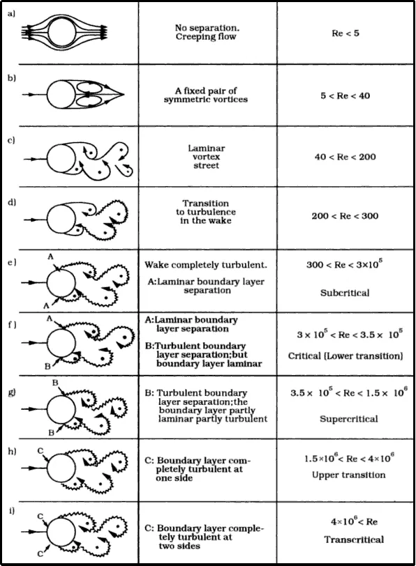
As the value of the Reynolds number is progressively incremented, the viscous effects gradually weaken, and fluid inertia increases, and naturally, a fluid element is no longer able to negotiate the sudden changes in body shape without incurring losses in its momentum (or kinetic energy). Therefore, a point is reached when due to the diverging area, an adverse pressure gradient is established in the rear of the cylinder thereby leading to the detachment of flow to the surface of the cylinder. The location of the point of separation coincides with that of the change of the sign of the velocity on the surface of the cylinder
The following figure shows the schematics of the different flow regimes past an unconfined circular cylinder.
Karman vortex street
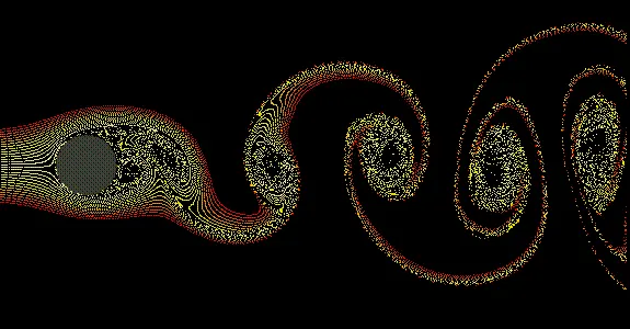
In fluid dynamics, a Karman vortex street is a repeating pattern of swirling vortices, caused by a process known as vortex shedding, which is responsible for the unsteady separation of flow of a fluid around blunt bodies.
A vortex street will form only at a certain range of flow velocities, specified by a range of Reynolds numbers (Re), typically above a limiting Re value of about 90. The (global) Reynolds number for a flow is a measure of the ratio of inertial to viscous forces in the flow of a fluid around a body or in a channel and may be defined as a nondimensional parameter of the global speed of the whole fluid flow.
Geometry Creation:-
From this point, we can start our project by creating our geometry in space claim using given dimensions.
2. Strouhal number:
In dimensional analysis, the Strouhal number is a dimensionless number describing oscillating flow mechanisms.
For large Strouhal numbers (order of 1), viscosity dominates fluid flow, resulting in a collective oscillating movement of the fluid "plug". For low Strouhal numbers (order of 10−4 and below), the high-speed, quasi-steady-state portion of the movement dominates the oscillation. Oscillation at intermediate Strouhal numbers is characterized by the buildup and rapidly subsequent shedding of vortices.
The Strouhal number is often given as
St=fDU′">`St=f*(D/U)`
Where,
f= frequency of vortex shedding
D= characteristic diameter of the cylinder
U'= fluid flow velocity
3. Co-efficient of drag:
In fluid dynamics, the drag coefficient(Cd)">(Cd) is a dimensionless quantity that is used to quantify the drag or resistance of an object in a fluid environment, such as air or water. It is used in the drag equation in which a lower drag coefficient indicates the object will have a less aerodynamic or hydrodynamic drag. The drag coefficient is always associated with a particular surface area.
The drag coefficient of any object comprises the effects of the two basic contributors to fluid dynamic drag: skin friction and form drag. The drag coefficient of a lifting airfoil or hydrofoil also includes the effects of lift-induced drag. The drag coefficient of a complete structure such as an aircraft also includes the effects of interference drag.
The drag coefficient Cd">Cd is defined as
`Cd=(2⋅Fd)/(ρu^2A)``
where:
- Fdis the drag force, which is by definition the force component in the direction of the flow velocity,
- ρ is the mass density of the fluid,
- uis the flow speed of the object relative to the fluid,
- A is the reference area.
4. Co-efficient of lift:
The lift coefficient (CL">CL) is a dimensionless coefficient that relates the lift generated by a lifting body to the fluid density around the body, the fluid velocity, and an associated reference area. A lifting body is a foil or a complete foil-bearing body such as a fixed-wing aircraft. CL is a function of the angle of the body to the flow, its Reynolds number, and its Mach number. The section lift coefficient cl refers to the dynamic lift characteristics of a two-dimensional foil section, with the reference area replaced by the foil chord.
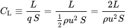
where
 is the lift force,
 is the relevant surface area and
q is the fluid dynamic pressure, in turn, linked to the fluid density, and to the flow speed.
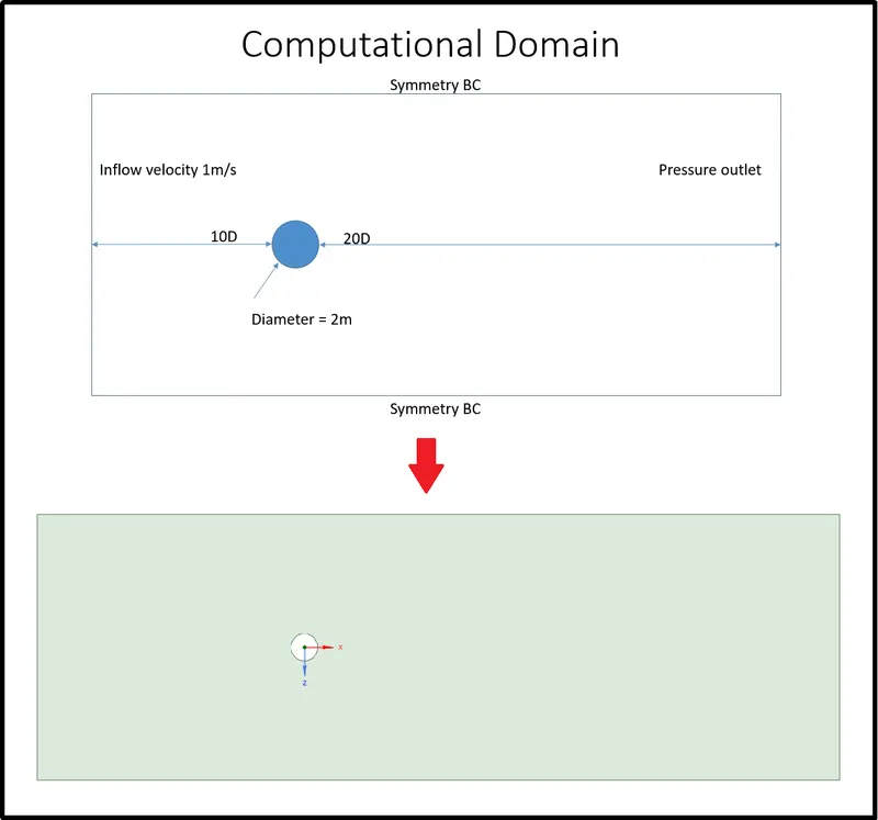
Geometry Creation:-
From this point, we can start our project by creating our geometry in space claim using given dimensions.
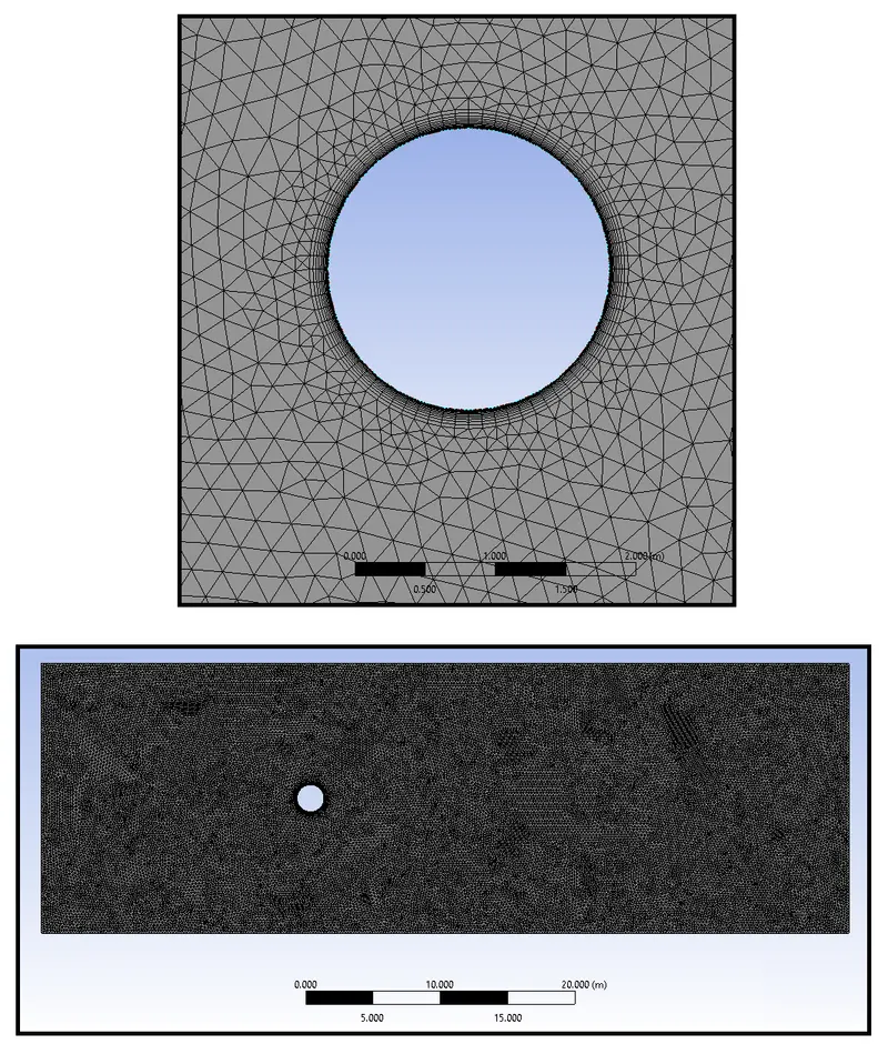
Meshing :
In meshing we are using triangular mesg method and the element size we have given here is 0.5.
we have selected the edge sizing option here to get the exact shape of the circle to capture all the physical properties over the cylinder.we are dividing into 36 equal distance layers of the circular geometry so that we can easily get the exact circle shape.
finally we are creating inflation layer on the cirle where the flow is happening.The first layer thickness as 0.005 and the increment of 1.2 times of 20 layers
finally we have set the initial and boundary layers of the geometry
SETUP :
Aim :
To Simulate the flow over a cylinder and explain the phenomenon of Karman vortex street.
Objectives :
PART-I
- Simulate the flow with the steady and unsteady case and calculate the Strouhal Number for Re= 100.
PART-II
- Calculate the coefficient of drag and lift over a cylinder by setting the Reynolds number to 10,100,1000,10000 & 100000. (Run with steady solver)
- Discuss the effect of Reynolds number on the coefficient of drag. [ Results should be validated with any standard literature and error should be within 5 %]
Expected results:-
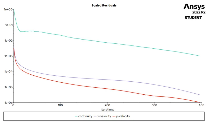
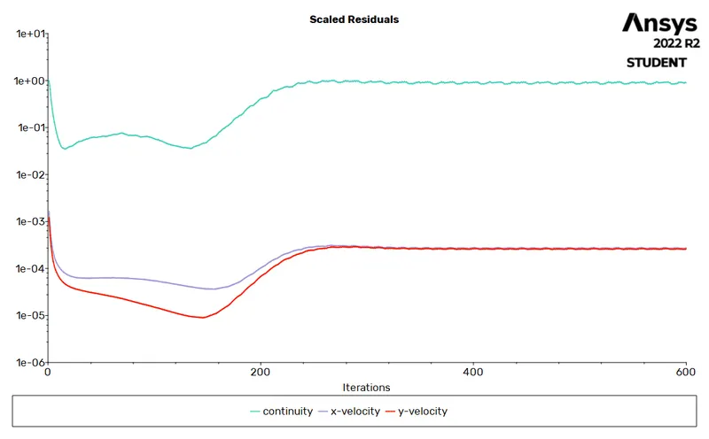
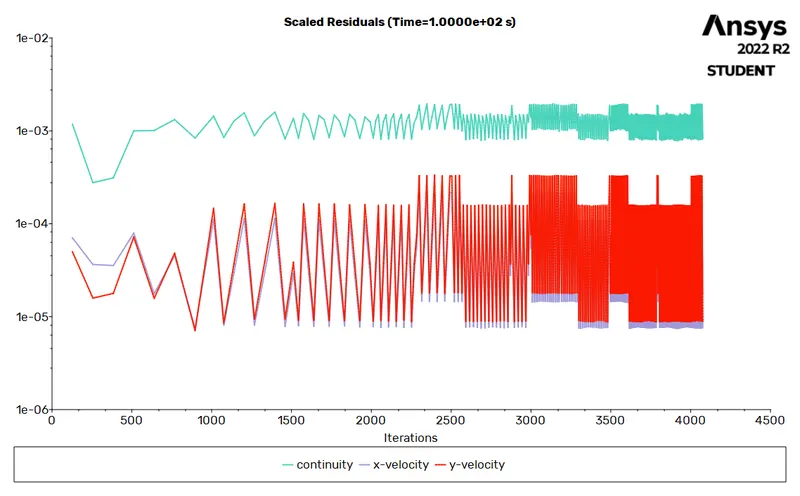
- In both approaches, show that the flow has converged. That is, what quantities or plots need to be looked at to determine that the flow has converged?
- Plots of the coefficient of drag and lift.
- Plots to show vortex shedding behind the cylinder.
- Mention the referred material (Reference Paper or Fluid Mechanics Textbook) at the end of the challenge submission page.
1. Flow over cylinder:
- In spite of extensive experimental and numerical studies almost over a century, flow around a circular cylinder still remains a challenging problem in fluid mechanics, where intensive investigations are continued even today to understand the complex unsteady dynamics of the cylinder wake flow.
- Cross-flow normal to the axis of a stationary circular cylinder and the associated problems of heat and mass transport are encountered in awide variety of engineering applications. Both experimental measurements and numerical computations have confirmed the onset of instability of the wake flow behind a cylinder beyond a critical Reynolds number, leading finally to a kind of periodic flow identified by definite frequencies, well-known in the literature as the Von Karman vortex street.
- In case of laminar flow past cylinders with regular polygonal cross-section, the flowusually separates at one or more sharp corners of the cross-section geometry itself, forming a system of vortices in the wake on either side of the mid symmetry plane.
- On the other hand, for a circular cylinder, where the point of flow separation is decided by the nature of the upstream boundary layer, the physics of the flow is much more complex than what its relatively simple shape might suggest.
This report emphasis on the analysis of two-dimensional flow over a circular cylinder in different Reynolds number. The analytical solution of the same case modeled with the potential flow is known and easy to interpret; however, the physical mechanism which rules real flow around a circular cylinder, as well as its mathematical treatment, is highly complex. Some examples are the boundary layer detachment and oscillatory effects that without a CFD study would be very difficult to determine either analytically or experimentally.
The unconfined or free flow past a circular cylinder exhibits a rich variety of flow regimes depending upon the intrinsic nature of the flow. It needs to be emphasized here that at finite Reynolds number, two flow regimes can be identified in the vicinity of the cylinder, i.e., the boundary layer of thickness, which is usually much smaller than the diameter of the cylinder and the wake region which is of the order of one-to-two times the diameter. Notwithstanding the fundamental significance of delineating the conditions for the transition from one flow regime to another, this information is also germane to develop the scaling laws for the gross engineering parameters like drag and lift coefficients, Strouhal number, and Nusselt number with the Reynolds number and Prandtl number. Therefore, significant research effort has been expended on exploring this aspect in this field. It is thus instructive to recapitulate the key points pertaining to the onset and distinguishing features of various flow regimes documented for the uniform transverse flow of Newtonian fluids past an unconfined smooth circular cylinder which is long in the transverse direction thereby eliminating the complications arising from the surface roughness and end effects, respectively.
For the aforementioned simple flow, the flow is governed by the familiar Reynolds number.
ReL=ULvo">`ReL=ULvoReL=ULvo`
Where,
U = the free stream flow speed.
L = a characteristic length parameter of the body or channel
vo">vovo = the free stream kinematic viscosity parameter of the fluid
vo=μoρ0">`vo=μoρ0vo=μoρ0`
ρ">ρρ = fluid density
μo">μoμo = dynamic viscosity
As the value of the Reynolds number is progressively incremented, the viscous effects gradually weaken, and fluid inertia increases, and naturally, a fluid element is no longer able to negotiate the sudden changes in body shape without incurring losses in its momentum (or kinetic energy). Therefore, a point is reached when due to the diverging area, an adverse pressure gradient is established in the rear of the cylinder thereby leading to the detachment of flow to the surface of the cylinder. The location of the point of separation coincides with that of the change of the sign of the velocity on the surface of the cylinder
The following figure shows the schematics of the different flow regimes past an unconfined circular cylinder.
Karman vortex street
In fluid dynamics, a Karman vortex street is a repeating pattern of swirling vortices, caused by a process known as vortex shedding, which is responsible for the unsteady separation of flow of a fluid around blunt bodies.
A vortex street will form only at a certain range of flow velocities, specified by a range of Reynolds numbers (Re), typically above a limiting Re value of about 90. The (global) Reynolds number for a flow is a measure of the ratio of inertial to viscous forces in the flow of a fluid around a body or in a channel and may be defined as a nondimensional parameter of the global speed of the whole fluid flow.
Geometry Creation:-
From this point, we can start our project by creating our geometry in space claim using given dimensions.
2. Strouhal number:
In dimensional analysis, the Strouhal number is a dimensionless number describing oscillating flow mechanisms.
For large Strouhal numbers (order of 1), viscosity dominates fluid flow, resulting in a collective oscillating movement of the fluid "plug". For low Strouhal numbers (order of 10−4 and below), the high-speed, quasi-steady-state portion of the movement dominates the oscillation. Oscillation at intermediate Strouhal numbers is characterized by the buildup and rapidly subsequent shedding of vortices.
The Strouhal number is often given as
St=fDU′">`St=f*(D/U)`
Where,
f= frequency of vortex shedding
D= characteristic diameter of the cylinder
U'= fluid flow velocity
3. Co-efficient of drag:
In fluid dynamics, the drag coefficient(Cd)">(Cd) is a dimensionless quantity that is used to quantify the drag or resistance of an object in a fluid environment, such as air or water. It is used in the drag equation in which a lower drag coefficient indicates the object will have a less aerodynamic or hydrodynamic drag. The drag coefficient is always associated with a particular surface area.
The drag coefficient of any object comprises the effects of the two basic contributors to fluid dynamic drag: skin friction and form drag. The drag coefficient of a lifting airfoil or hydrofoil also includes the effects of lift-induced drag. The drag coefficient of a complete structure such as an aircraft also includes the effects of interference drag.
The drag coefficient Cd">Cd is defined as
`Cd=(2⋅Fd)/(ρu^2A)``
where:
- Fdis the drag force, which is by definition the force component in the direction of the flow velocity,
- ρ is the mass density of the fluid,
- uis the flow speed of the object relative to the fluid,
- A is the reference area.
4. Co-efficient of lift:
The lift coefficient (CL">CL) is a dimensionless coefficient that relates the lift generated by a lifting body to the fluid density around the body, the fluid velocity, and an associated reference area. A lifting body is a foil or a complete foil-bearing body such as a fixed-wing aircraft. CL is a function of the angle of the body to the flow, its Reynolds number, and its Mach number. The section lift coefficient cl refers to the dynamic lift characteristics of a two-dimensional foil section, with the reference area replaced by the foil chord.
where
is the lift force,
is the relevant surface area and
q is the fluid dynamic pressure, in turn, linked to the fluid density, and to the flow speed.
Geometry Creation:-
From this point, we can start our project by creating our geometry in space claim using given dimensions.
Meshing :
In meshing we are using triangular mesg method and the element size we have given here is 0.5.
we have selected the edge sizing option here to get the exact shape of the circle to capture all the physical properties over the cylinder.we are dividing into 36 equal distance layers of the circular geometry so that we can easily get the exact circle shape.
finally we are creating inflation layer on the cirle where the flow is happening.The first layer thickness as 0.005 and the increment of 1.2 times of 20 layers
finally we have set the initial and boundary layers of the geometry
SETUP :
| SL.NO | for all the cases except unsteady case same setup we have used | |
| 1 | solver | steady state |
| 2 | energy equation | off |
| 3 | model | laminar |
| 4 | inlet | velocity inlet |
| 5 | outlet | pressure outlet |
| 6 | fluid (material) | user defined |
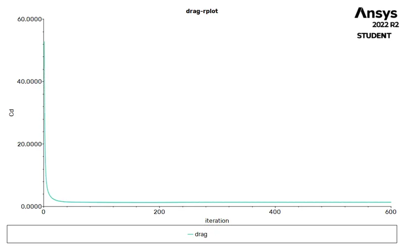
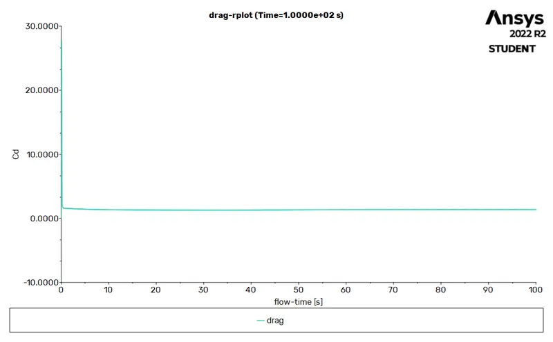
Here we are using the geometry to simulate by varying the reynolds number interms of incresing the velocity.
We are running the simulation with steady state in all the simulations.
ALL THE GRAPHS ARE IN THIS OREDER
Reynolds number velocity
1) Re -10 0.25m/s
2) Re -100 2.5m/s
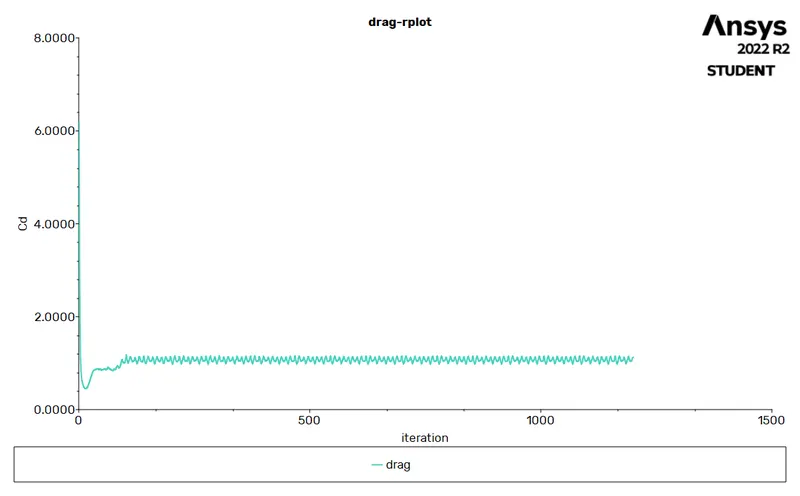
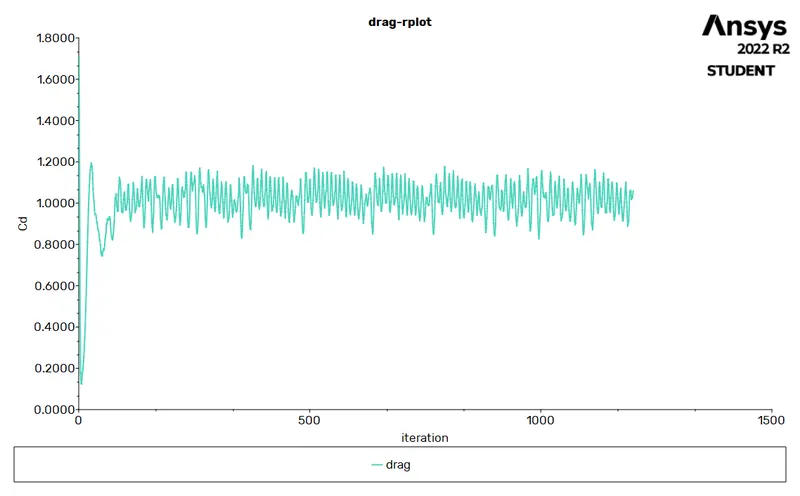
3) Re -100(unsteady) 2.5m/s
4) Re -1000 25m/s
5) Re -10000 250m/s
6) Re -100000 2500m/s
I am comparing all the results in one on one for the better visualisation and also to compare better
RESIDUAL PLOTS :
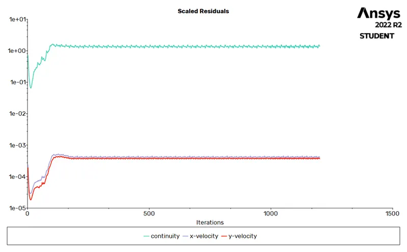
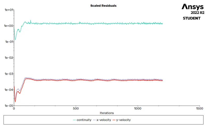
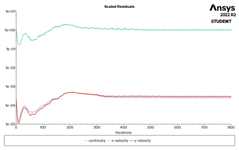
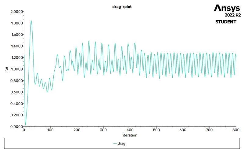
DRAG FORCE :
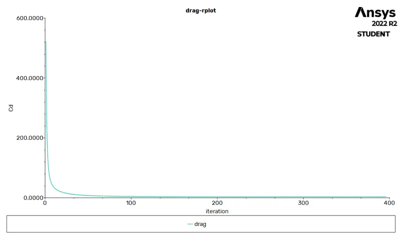
LIFT FORCE :
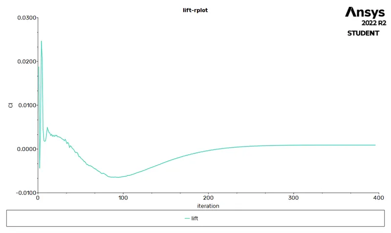
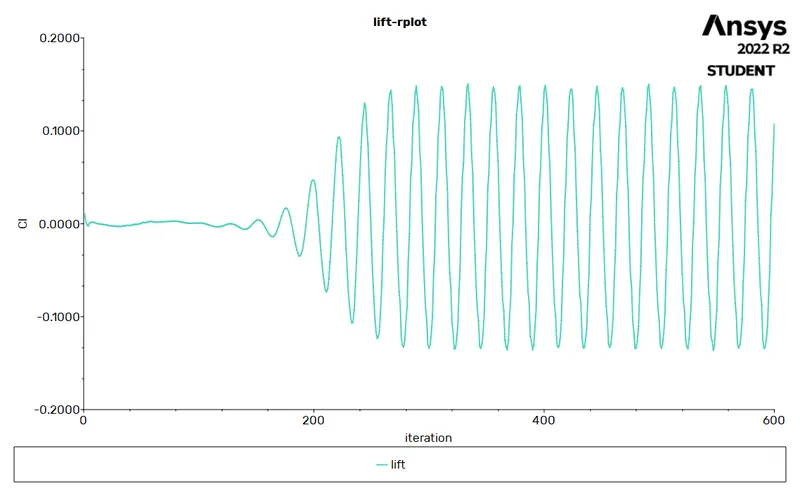
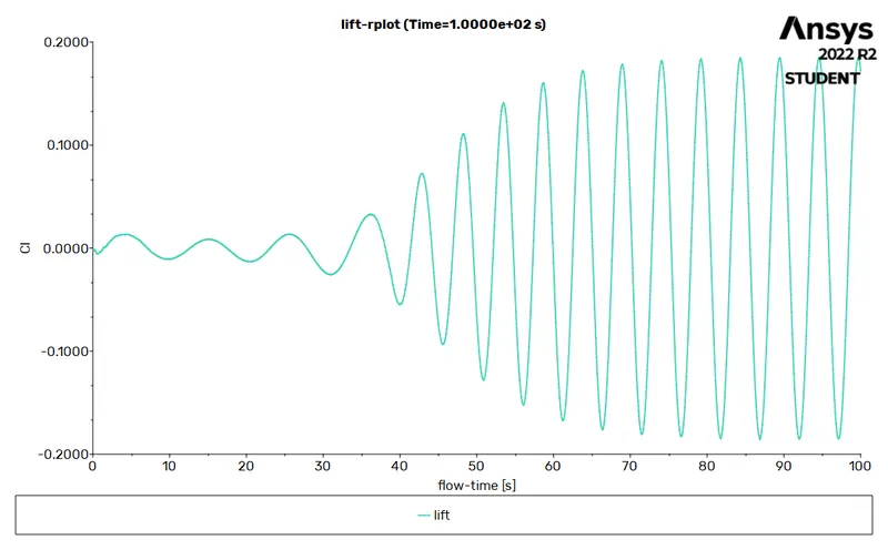
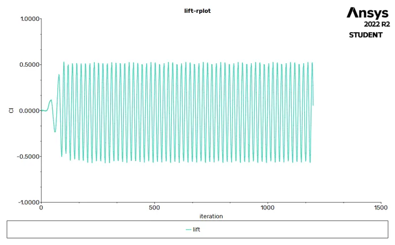
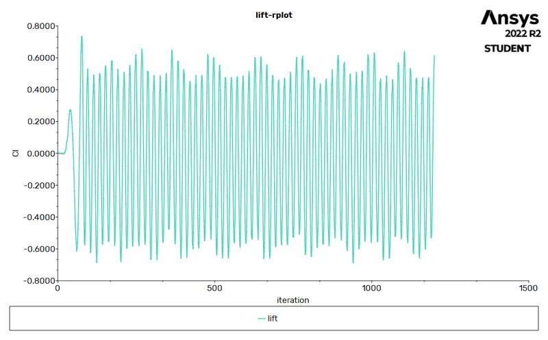
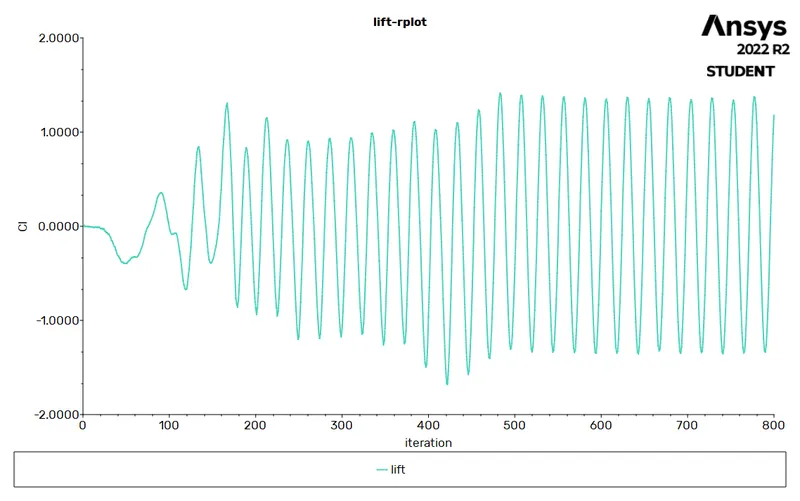
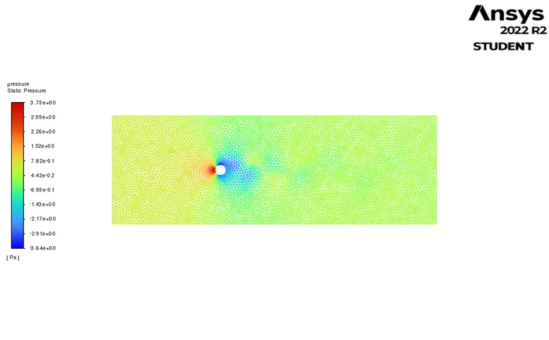
VERTEX SHEDDING :
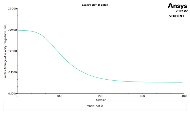
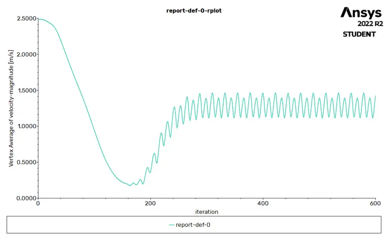
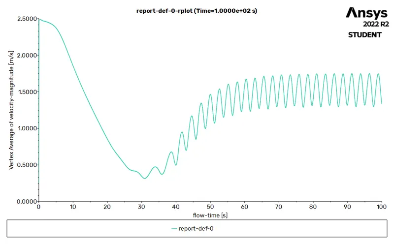
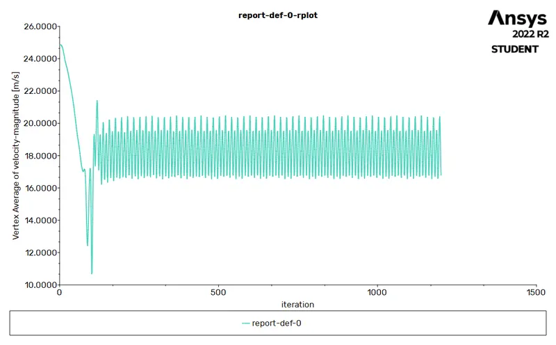
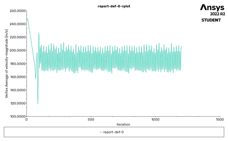
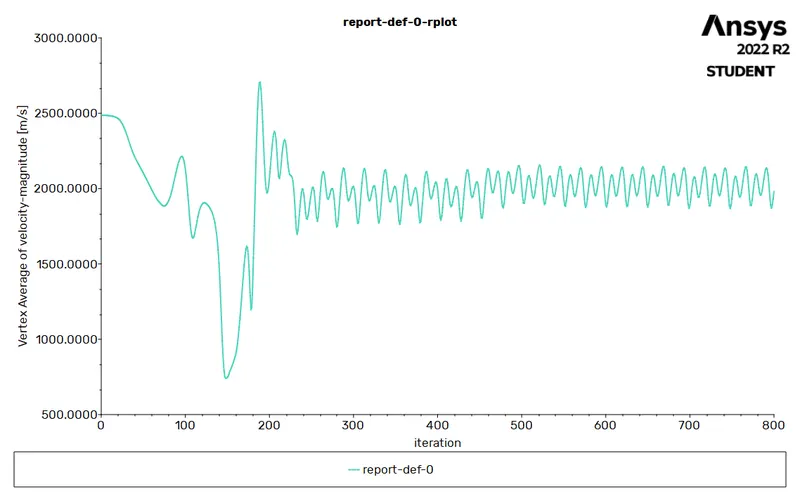
RE -10
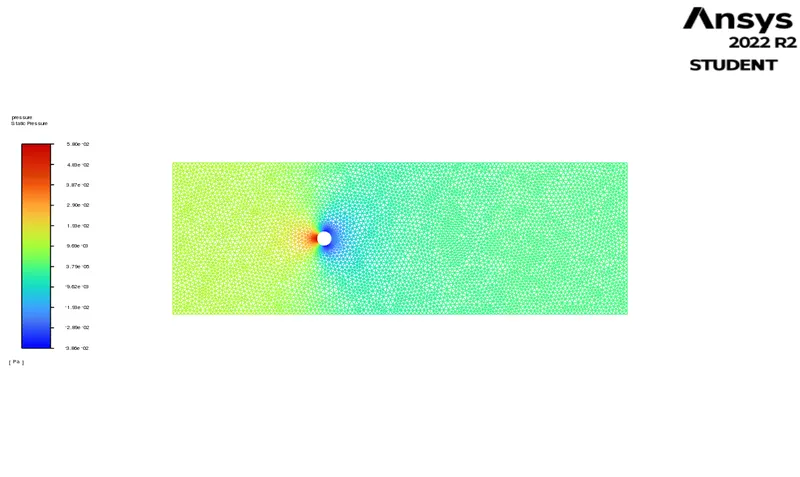
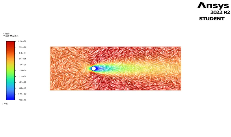
RE -100
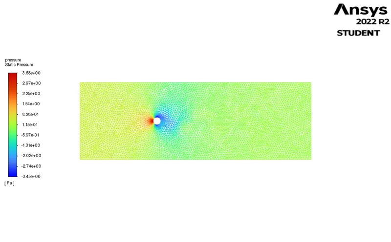
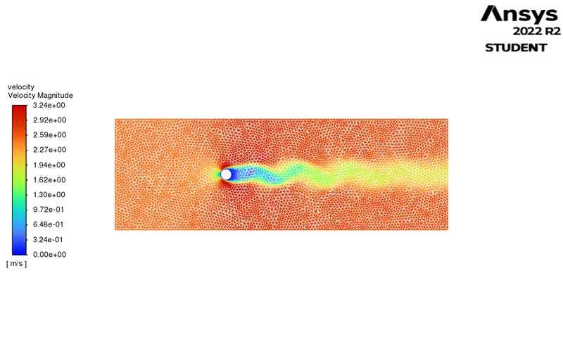
RE-1000
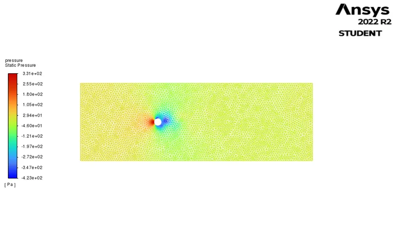
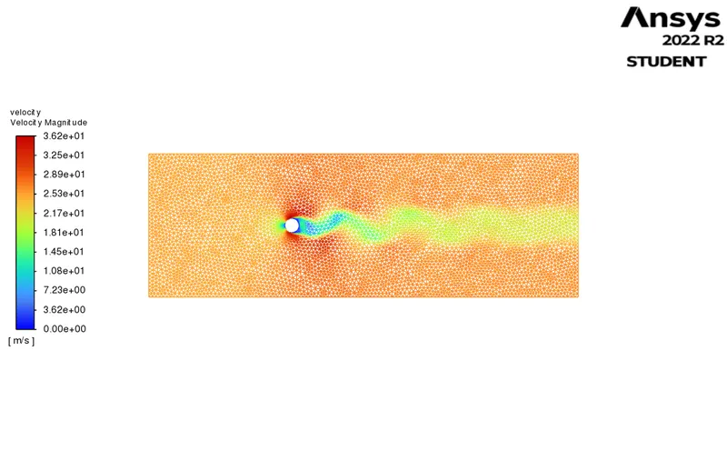
Re-10000
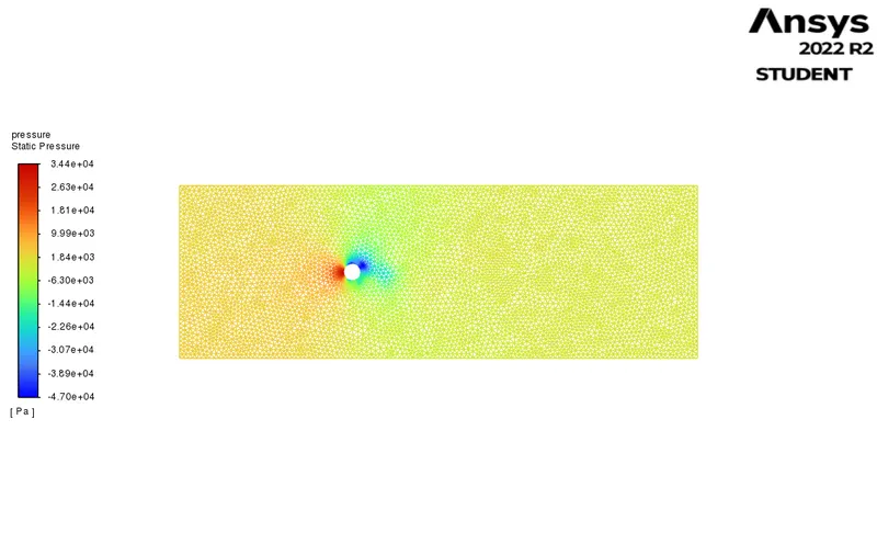
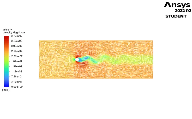
Re - 100000
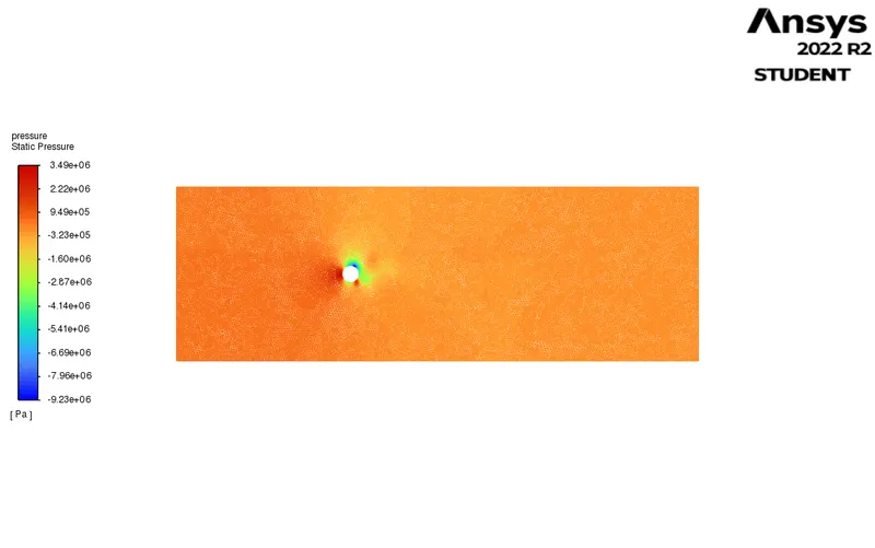
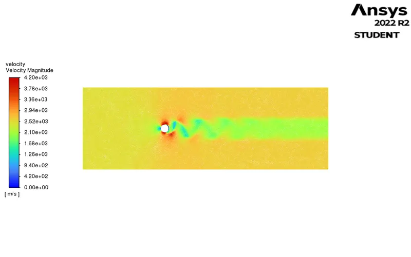
Re-100(unsteady)
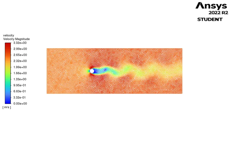
strouhal number -100(unsteady)
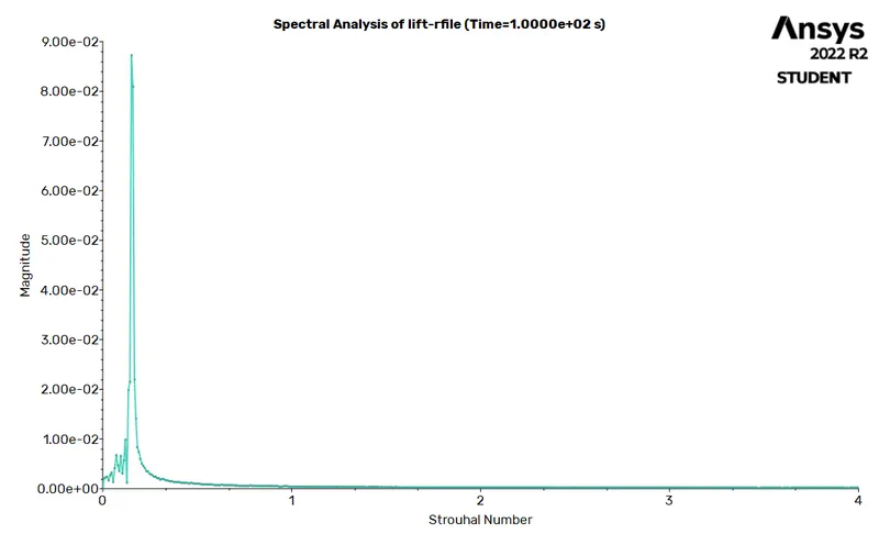
the strouhal number of the unstaedy state for 100 reylolds number is 0.001
max strouhal number is is 0.08
when we compare the above grapgs as per the problem statement
| Reynolds number | drag coefficient | lift coefficient | vortex shedding |
| 10 | 3.32 | 0.000899 | 0.126 |
| 100 | 1.33 | 0.133 | 1.42 |
| 1000 | 1.124 | 0.5688 | 18.00 |
| 10000 | 1 | 0.6149 | 185 |
| 100000 | 0.84 | 1.1908 | 1988 |
| 100 (unsteady) | 1.345 | 0.138 | 1.43 |
| Reynolds number | theoretical Cd | Numerical Cd | error |
| 10 | 3.5 | 3.333 | 4.77% |
| 100 | 1.4 | 1.333 | 2.5% |
Conclusions:
- In the first case, the flow over a cylinder is simulated for both unsteady cases with Re=100, and with the results generated the phenomena of Von Karman Vortex Street are also observed.
- Necessary plots are plotted in order to observe that the flow is converged and the vortex shedding is happening.
- Contours are generated in order to observe the flow over a cylinder.
- By plotting Power Spectral Density vs Frequency, the Strouhal number is calculated.
- In the second case,
- six different simulations i.e (Re = 10,100,1000,10000,100000,1000000) are simulated to observe the behavior of the drag and lift coefficients by changing the Reynolds number.
- In order to observe the behavior of the drag coefficients for the simulations, the velocity of the flow is varied to change the Reynolds number and the rest of the parameters are kept constant.
- As we know if the Reynold number is less than 100000, then flow in a pipe is Laminar for external flow. Hence we use the Viscous model = Laminar.
- For Re=10, it is observed that there is no formation of vortex shedding and in the rest of the cases, it is clearly observed.
- As per the basic conditions and parameters, the results are validated from the literature.
- As we refine the mesh we need to run more iterations.
- From the above table, it can be concluded that the error percentage is less than 5%.
| SL.NO | PROERTY | |
| 1 | ||
| 2 | ||
| 3 | ||
| 4 | ||
| 5 | ||
| 6 | ||
| 7 | ||
| 8 | ||
| 9 |
Here we are using the geometry to simulate by varying the reynolds number interms of incresing the velocity.
We are running the simulation with steady state in all the simulations.
ALL THE GRAPHS ARE IN THIS OREDER
Reynolds number velocity
1) Re -10 0.25m/s
2) Re -100 2.5m/s
3) Re -100(unsteady) 2.5m/s
4) Re -1000 25m/s
5) Re -10000 250m/s
6) Re -100000 2500m/s
I am comparing all the results in one on one for the better visualisation and also to compare better
RESIDUAL PLOTS :
DRAG FORCE :
LIFT FORCE :
VERTEX SHEDDING :
RE -10
RE -100
RE-1000
Re-10000
Re - 100000
Re-100(unsteady)
strouhal number -100(unsteady)
when we compare the above grapgs as per the problem statement
| Reynolds number | drag coefficient | lift coefficient | vortex shedding |
| 10 | 3.32 | 0.000899 | 0.126 |
| 100 | 1.33 | 0.133 | 1.42 |
| 1000 | 1.124 | 0.5688 | 18.00 |
| 10000 | 1 | 0.6149 | 185 |
| 100000 | 0.84 | 1.1908 | 1988 |
| 100 (unsteady) | 1.345 | 0.138 | 1.43 |
| Reynolds number | theoretical Cd | Numerical Cd | error |
| 10 | 3.5 | 3.333 | 4.77% |
| 100 | 1.4 | 1.333 | 2.5% |
Conclusions:
- In the first case, the flow over a cylinder is simulated for both Steady and unsteady cases with Re=100, and with the results generated the phenomena of Von Karman Vortex Street are also observed.
- Necessary plots are plotted in order to observe that the flow is converged and the vortex shedding is happening.
- Contours are generated in order to observe the flow over a cylinder.
- By plotting Power Spectral Density vs Frequency, the Strouhal number is calculated.
- In the second case,
- six different simulations i.e (Re = 10,100,1000,10000,100000,1000000) are simulated to observe the behavior of the drag and lift coefficients by changing the Reynolds number.
- In order to observe the behavior of the drag coefficients for the simulations, the velocity of the flow is varied to change the Reynolds number and the rest of the parameters are kept constant.
- As we know if the Reynold number is less than 100000, then flow in a pipe is Laminar for external flow. Hence we use the Viscous model = Laminar.
- For Re=10, it is observed that there is no formation of vortex shedding and in the rest of the cases, it is clearly observed.
- As per the basic conditions and parameters, the results are validated from the literature.
- As we refine the mesh we need to run more iterations.
- From the above table, it can be concluded that the error percentage is less than 5%.