Week 2 - Flow over a Cylinder.

Aim:- Simulate the flow over a cylinder and explain the Van karman vertex street.

Objective:- 1. Simulate the flow with the stready and unsteady cases and calculate the strouhal no for Re=100.

2. Calculate the coefficient of drag and lifer over a cylinder by setting the Reynolds no 10, 100, 1000, 10000 & 100000(run with steady solver). Discuss the effect of Reynolds number on the coefficient of drag.

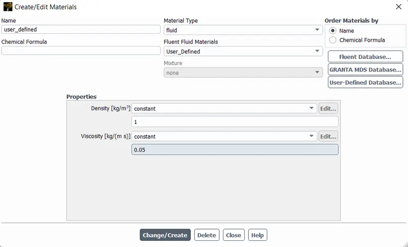
Introduction:- We are interested in simulating flow over cylinder to do this we are using a user defined materials as air but with density as 1 kg/m^3 and .05. We vary the reynolds no to understand the concept of vertex formation, negative pressure reason and effect of Reynolds no of flow. Our main study is focused in finding the vertex velocity at a given point named as monitor point along with this we are interested in calculating the strouhal no.

Theory:- There are mainly three type of flow

1. Laminar
2. Turbulent
3. Transient

To understand the type of flow we have a dimension less entity known as Reynolds no

Basic Formula is Re = Rho*V*L/miu

Rho is density, V is velocity, L is the length , miu is the dynamic viscosity

Type of Flow	Reynolds no.
	Internal	External
Laminar	<2400	<2*10^5
Turbulent	>4000	>5*10^5
Transient	2000<Re<4000	2*10^5<Re<5*10^5

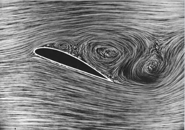
Van Karman Vertex Flow:- When fluid flows towards the body, the flow around a bluff body produces a regular pattern of alternating vortices known as van karman vertex flow. These vortices produce a sinusoidal force acting on the body in the perpendicular to the direction of flow. When we are analyzing flow over cylinder strouhal no. play a very vital role. Generally vertex shedding with laminar flow is considered as van karman vertex flow or when laminar flow with low reynolds no. produces periodic vortex.

Strouhal No. = frequency*diameter*/velocity

Here frequency related with the shedding formation.

Drag Force:- is a force acting opposite to the relative motion of any object moving with respect to a surrounding fluid. this force have a great significance in study of turbines.

Drag forces increases as the velovity of the fluid increases. as it show a direct proportional relation with square of velocity.

with increase in the frontal area drag force also increases.

General formula.

here rho is the denisy of the fluid

v is the velocity of the fluid

Cd is the drag coeeficient(with increase in reynolds no drag coefficient will decreases).

A is the frontal area

Lift Force:- Lift is the component of force that is perpendicular to the oncoming flow direction

Lift force icreases as the velovity of the fluid increases. as it show a direct proportional relation with square of velocity.

Lift force and Drag force are perpendicular to each other

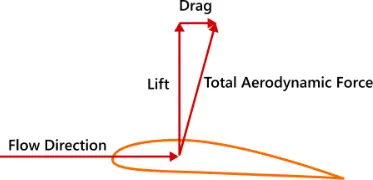
Flow Sepration:-flow separation or boundary layer separation is the detachment of a boundary layer from a surface into a wake. This is generally comes into picture when a fluid passing over a body or comes in contact with a solid surface or any sufaces.

Theroy:- Computational fluid dynamics or CFD is the analysis of systems involving fluid flow, heat transfer and associated phenomena such as chemical reactions by means of computer-based simulation.

Practical application in current scenario

• aerodynamics of aircraft and vehicles: lift and drag
• hydrodynamics of ships
• power plant: combustion in internal combustion engines and gas
turbines
• turbomachinery: flows inside rotating passages, diffusers etc.
• electrical and electronic engineering: cooling of equipment including
microcircuits
• chemical process engineering: mixing and separation, polymer moulding
• external and internal environment of buildings: wind loading and
heating/ventilation
• marine engineering: loads on off-shore structures
• environmental engineering: distribution of pollutants and effluents
• hydrology and oceanography: flows in rivers, estuaries, oceans
• meteorology: weather prediction
• biomedical engineering: blood flows through arteries and veins

CFD Work Flow:- CFD codes are structured around the numerical algorithms that can tackle fluid flow problems. In order to provide easy access to their solving power all commercial CFD packages include sophisticated user interfaces to input problem parameters and to examine the results

Its threee step process
(i) a pre-processor

involves defination of geometry, grid generation, selection of phenomenon that need to model

(ii) a solver

intergration of governing equation, discretisation and solution

(iii) a post-processor

ploting of contour, graphs and making movies.

In solving fluid flow problems we need to be aware that the underlyingphysics is complex and the results generated by a CFD code are at best asgood as the physics (and chemistry) embedded in it and at worst as good asits operator with CFD

Solving and Modeling Approch:-

There are no way present to understand and analyse the effeciveness of the mixiing tee model.

1. analytical approch

2. simulation approch

3. experimental approch

using analytical approch and experimental approch is time consuming and high cost senario. this could be eliminated by using simulation approch in which we can analyse the system with the actual codition we are intrested in.

To do this we are using ansys fluent solver

we are using fluid flow analysis using Fluent solver because we are interested in the total effectiveness of the fluid in the mechnical tee model, here we are using two different models to analyse the effectiveness of the mixing of fluid.

Mesh length choose as 500

Approch used

1. We need to open Ansys workbench

2. Choose the Appropiate Solver

3. Assign Appropiate name

4. Choose geometry and select new spaceclaim model.

5. Generate the model in spaceclaim itself

6. Implement the geometrical operation

7. Apply the mesh and provide name selection

8. Choose setup, select the appropiate model

9. Initalisation and running the simulation

10. Result making i.e. countour plots graphs

Choosing and geometry generation using spaceclaim

1. choose the fluid flow (fluent)

2. right click on the geometry choose new spaceclaim geometry

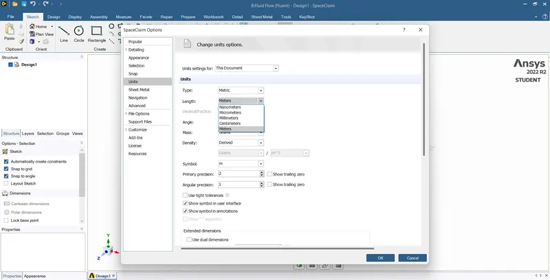
3. set the units in the required format

file>spaceclaim options>units>meters

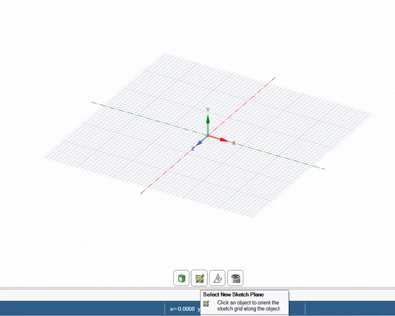
4. go to sketch mode

at bottom sketch>select the working plane(XY Plane)>press on z axis to get xy plane.

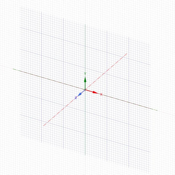
5. Draw a required geometry

cicrle of 2m diameter

rectangle or computational domain 20*60 meter^2

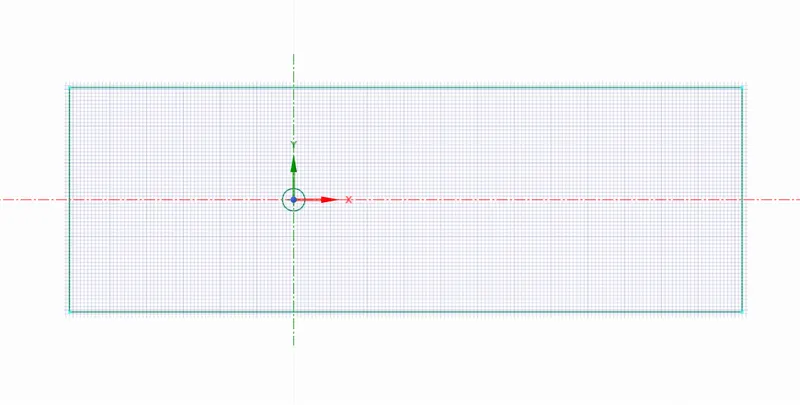
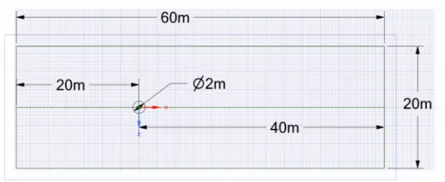
6. use pull command or return to 3d mode

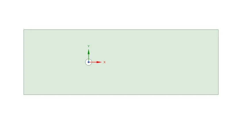
we created the geometry with computional domain.

now we move to our 2nd strep that is meshing

Meshing

now we open mesh window

1. click on the mesh and choose element length as 500mm i.e. .5m and click on generate mesh

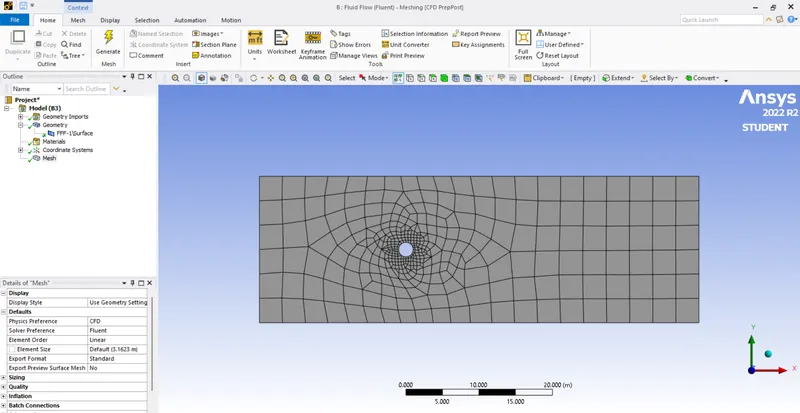
we set the element size as 500mm i.e. .5m and set the method from quadrilateral dominanto triangles

mesh>insert>methods>select the geometry>select apply(geometry became blue)>change method quadrilateral dominant to triangles

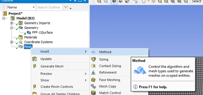
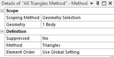
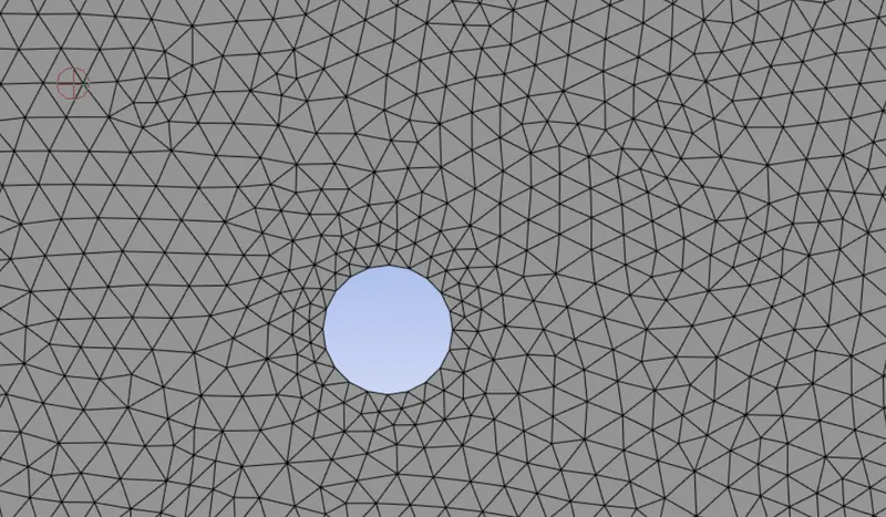
we observe that the cylinder or hole is not uniform, to make it uniform we use sizing option.

mesh>insert>sizing>select the edge>select apply>change type from element size to number of division.

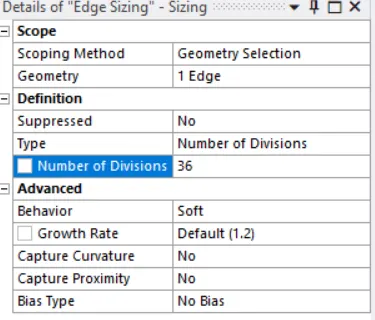
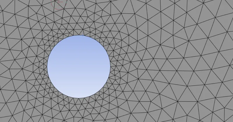
Now we are intrested in capturing the effect of working medium at the cylindical wall, to capture this perfectly we can create structured mesh near the cylindrical wall

mesh>insert>inflation>select the body>select the edge>choose frist layer thickness from inflation option>give frist layer thickness and no of layers

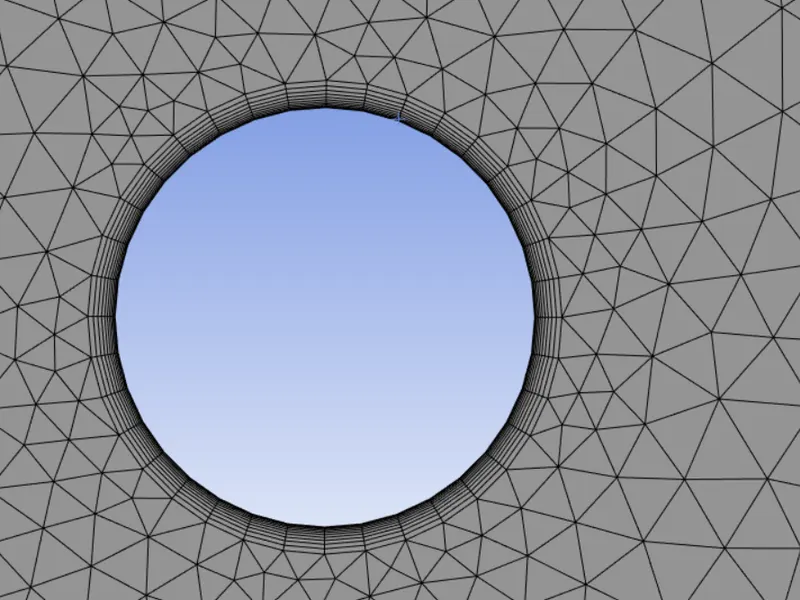
Now we can provide the name selection

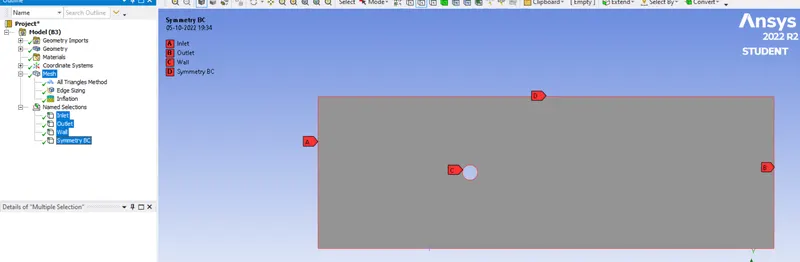
we end up with the mesh windonw.

Setup:-

Settings

Solver	Steady State
Energy Equation	Off
Model	Laminar
Inlet	Inlet Velocity
Outlet	Pressure Outlet
Material_(Fluid)	Air(User Defined Property)
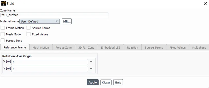
Cell Zone Condition	User Material
Boundary Condition	Velocity Input Based On Re

Solver, Model,

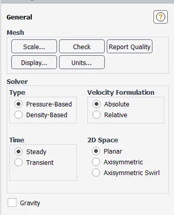
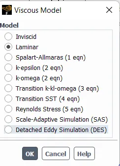
material

Cell zone condition

Inlet Velocity

Reynolds Number	Velocity (m/s)
10	.25
100	2.5
1000	25
10000	250
100000	2500

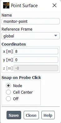
Setting Monitor Point

result>create>point>define name>define coordinates

Results Needed

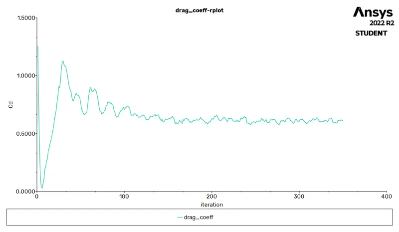
1. Drag Coefficient graph

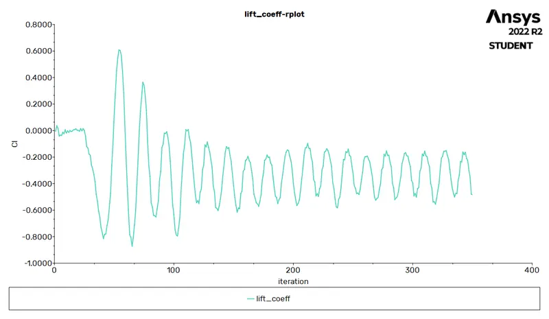
2. Lift Coefficient graph

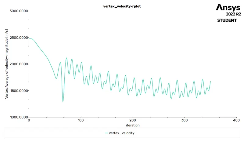
3. Vertex Velocity

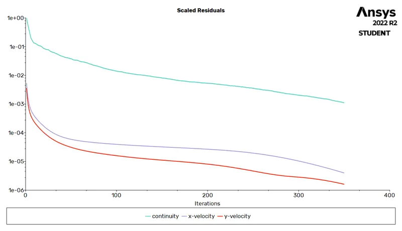
4. Residual Plot

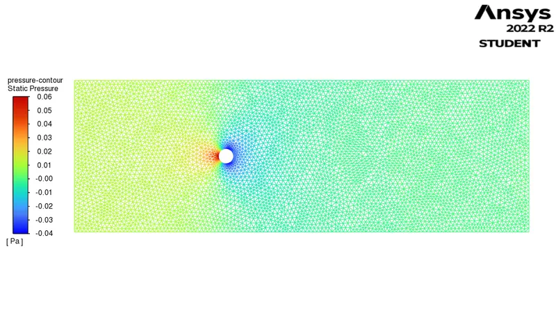
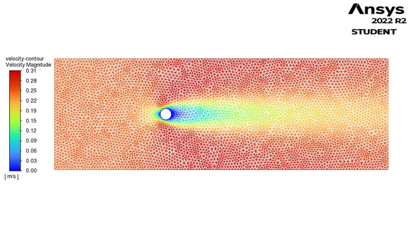
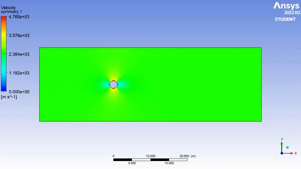
5. Velocity Contour

6. Pressure Contour

Result For Reynolds No 10

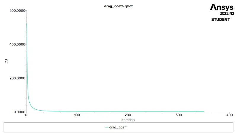
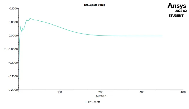
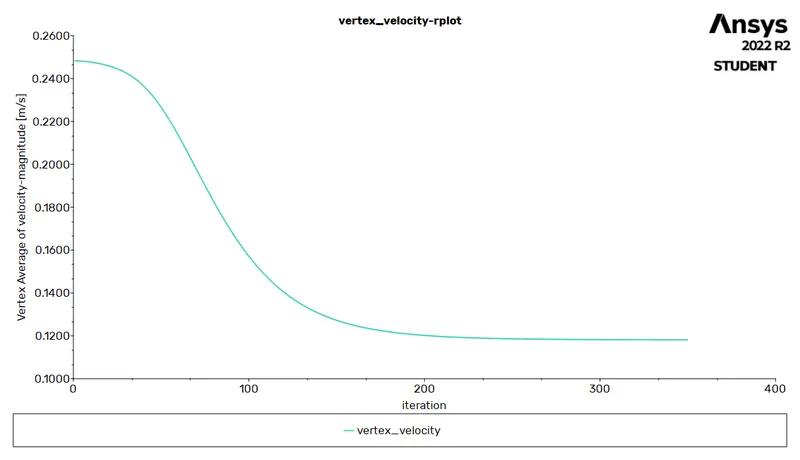
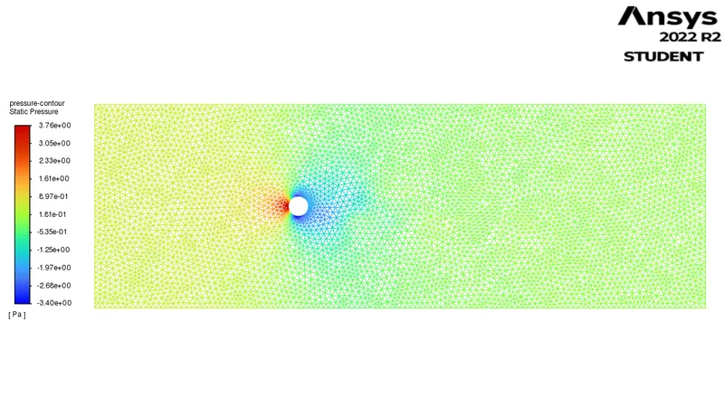
Result For Reynolds No 100

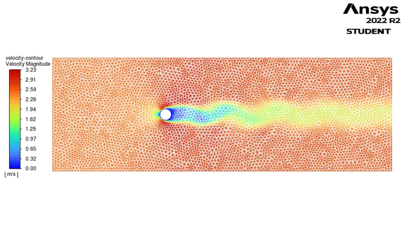
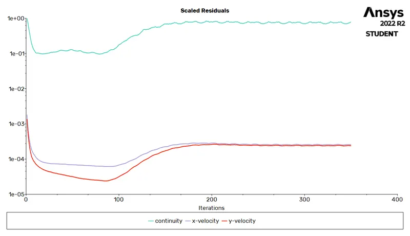
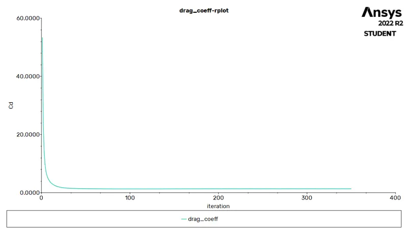
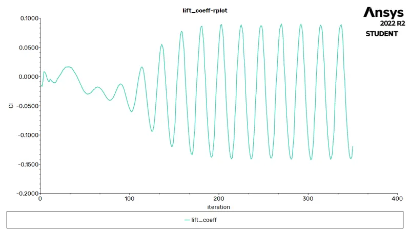
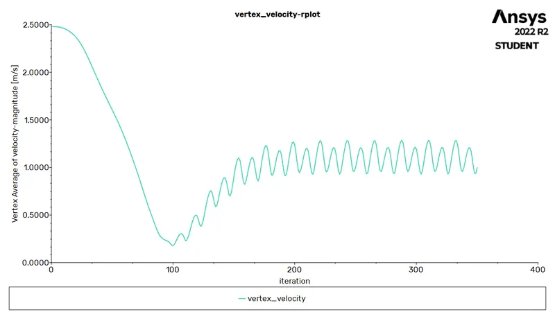
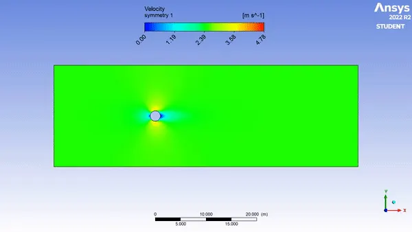
Strouhal Number:-

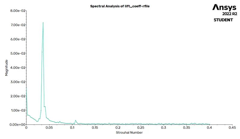
Strouhal No. is .071565

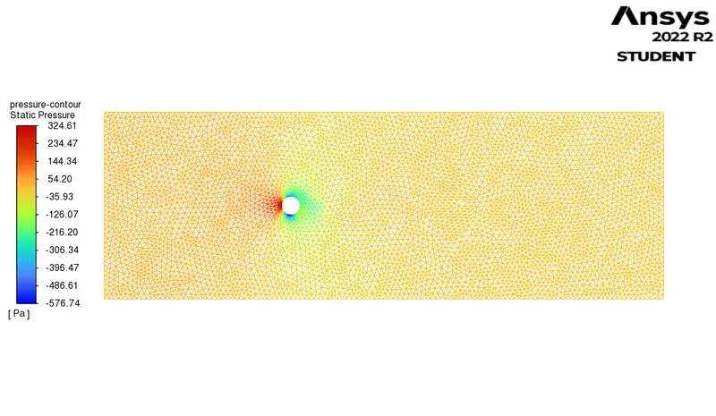
Result For Reynolds No 1000

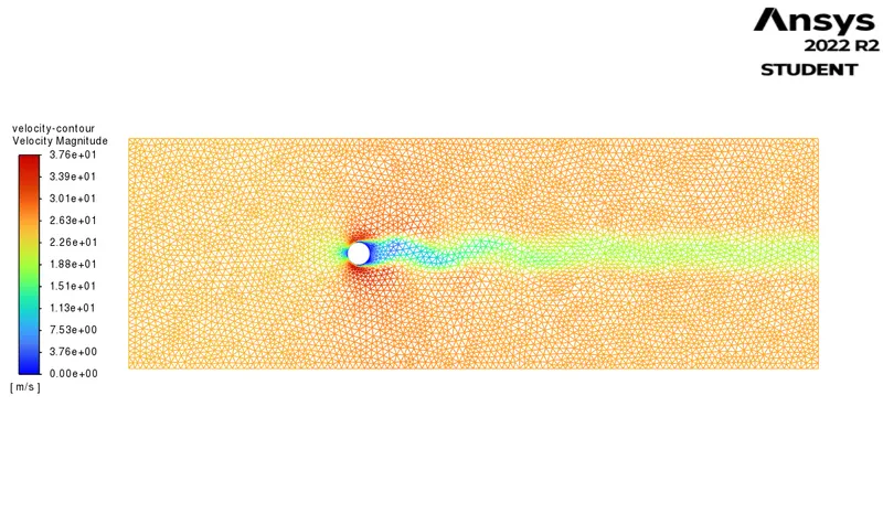
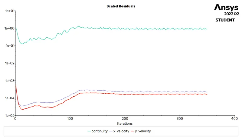
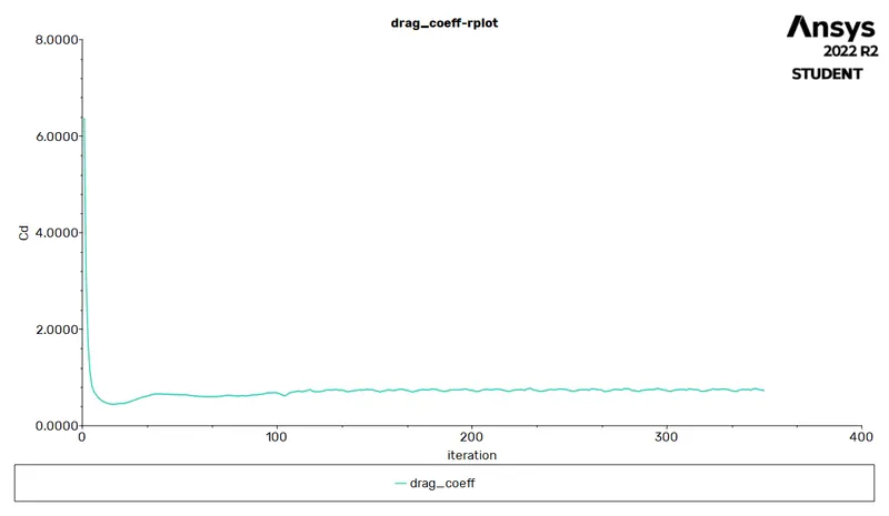
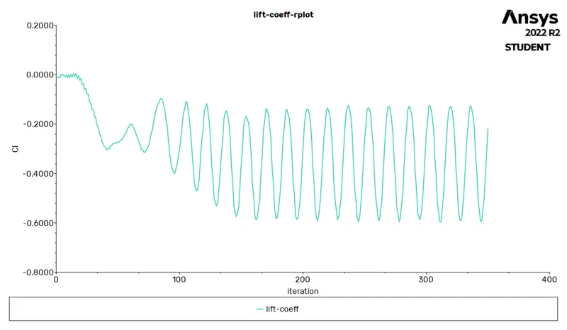
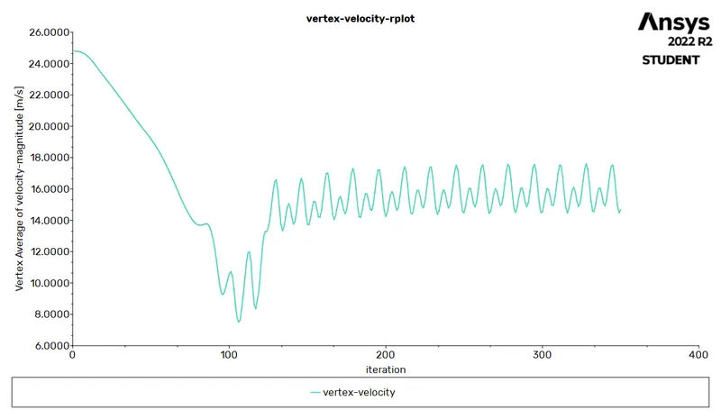
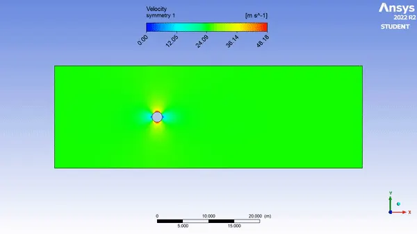
Result For Reynolds No 10000

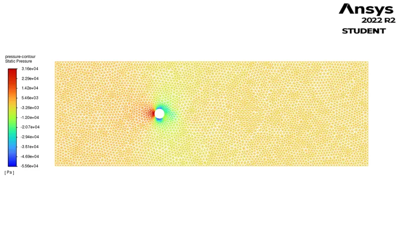
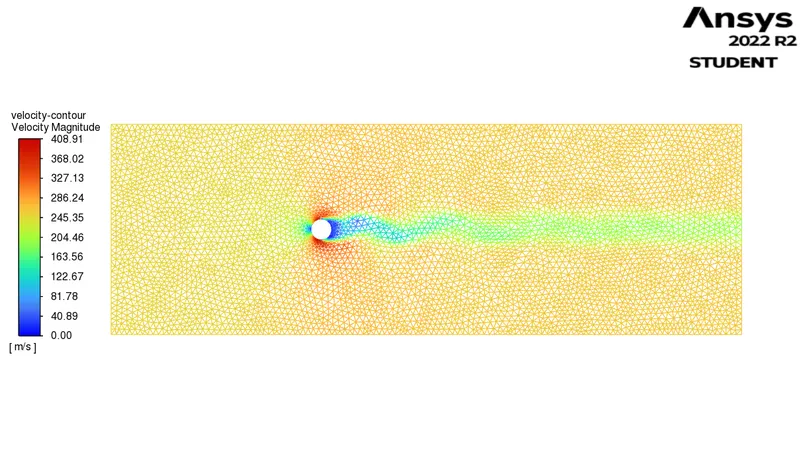
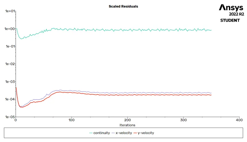
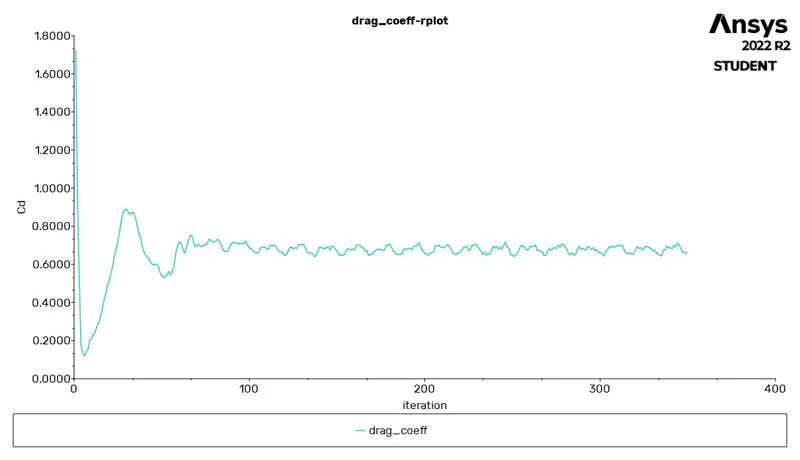
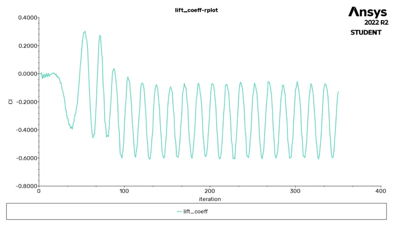
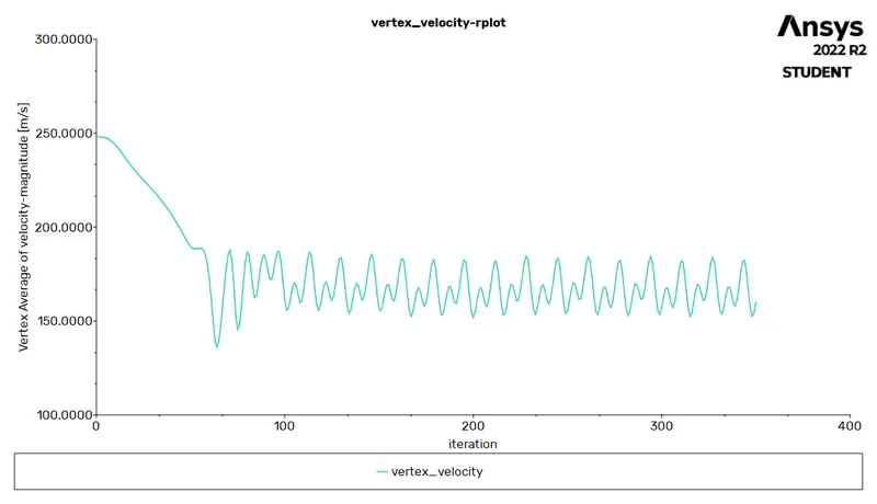
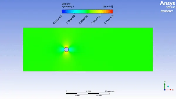
Result For Reynolds No 100000

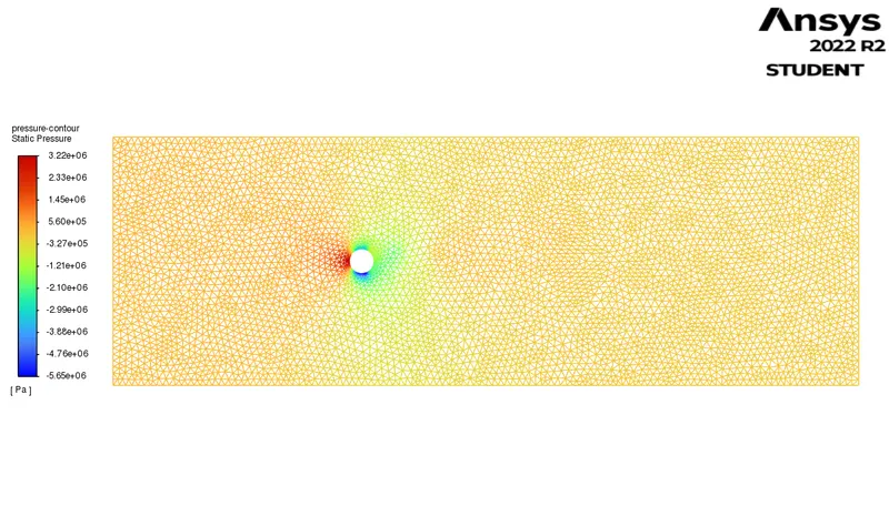
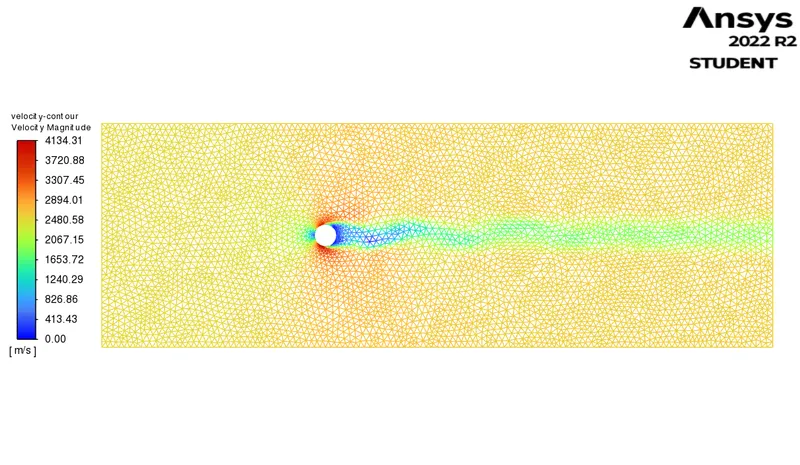
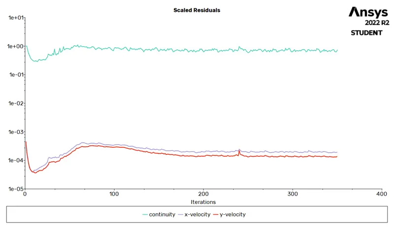
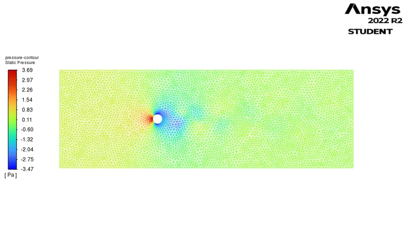
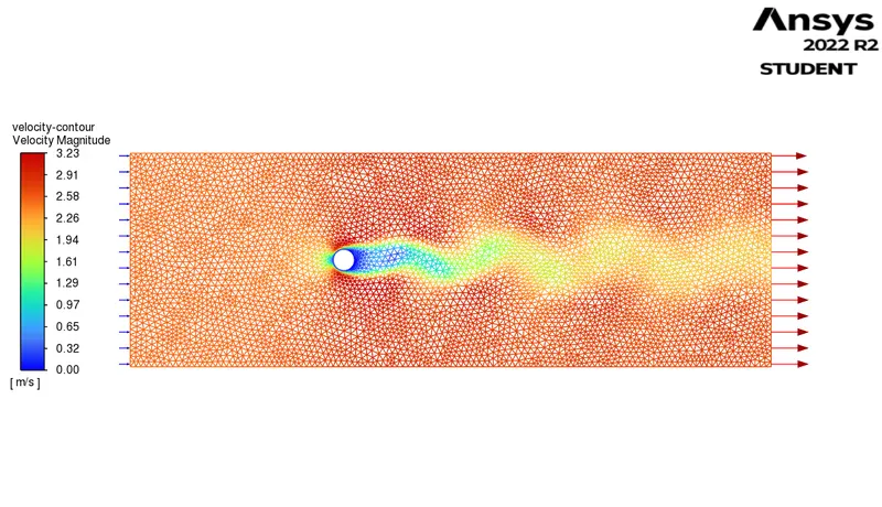
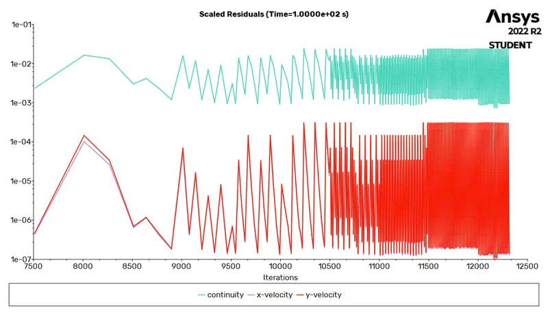
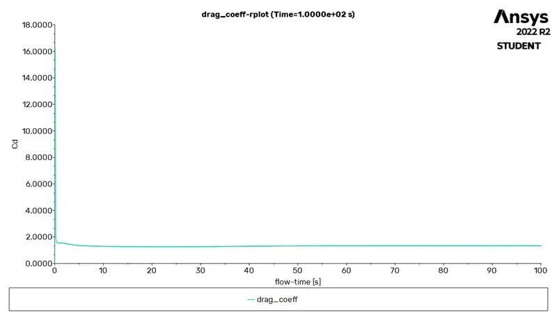
Tansient State

Reylonds No. 100, Velocity 2.5m/s, Time step size = .1, No of time steps = 1000

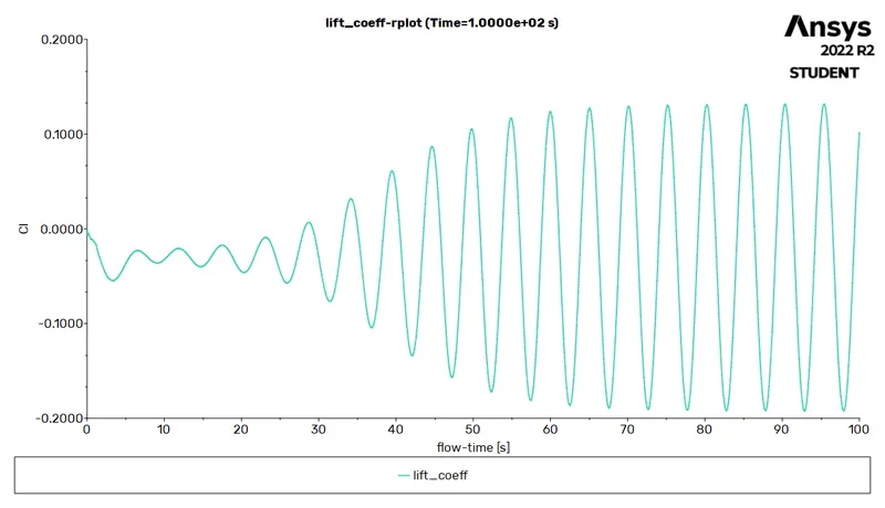
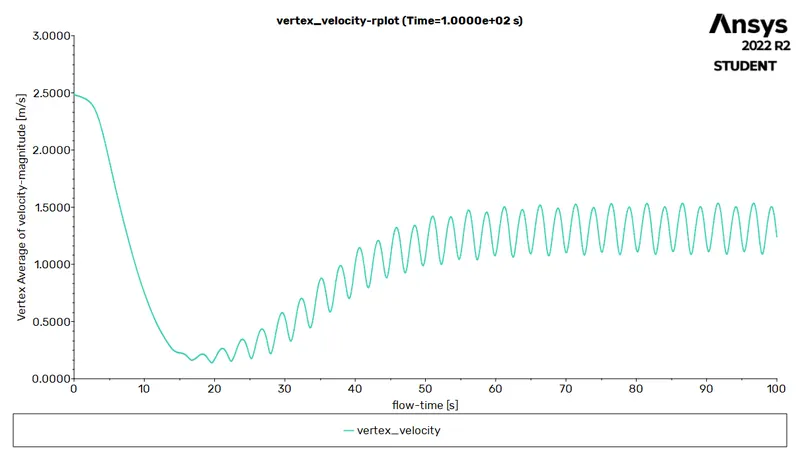
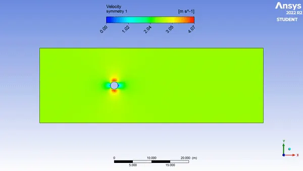
Stouhal No.

Finals Result:-

Reynolds Number	Drag Coefficient	Life Coefficient	Vertex Velocity
10	3.3123	-0.00164	0.1181
100	1.322	-0.1188	0.9973
1000	0.7236	-0.2173	14.6859
10000	0.6655	-0.1276	160.33
100000	0.609	-0.4862	1680.68

For Transient

Reynolds Number	Drag Coefficient	Life Coefficient	Vertex Velocity
100	1.333	0.101	1.24

Inferences:-

1. drag coefficient decreases with increase in the reynolds no.

2. as we move monitor point towards the right side we observe increase in velocity.

3. with increase in reynolds no. increases the chance of flow sepration

4. strouhal no. for steady state reynolds no. 100 is .071 and for unsteady state

5. weak region negative pressure region are formed behind the cylindrical body

6. pressure on the left side of cylinder is high because it is in direct contact

7. in transient state we are plotinh graphs w.r.t. to time instead of iteration.

8. velocity is nearby zero at left side of cylinder

9. pressure is high then velocity is low and vice versa

References:

https://www.sciencedirect.com/science/article/pii/S0307904X08000243

Aerodynamics : selected topics in the light of their historical development by Theodore von Karman.