Ansys - Flow over a Cylinder.
Problem Statement: -
For a 2m diameter Cylinder. Perform a CFD Simulation to Analyse Flow over the Cylinder for Reynolds Numbers 10, 100, 1000, 10000, 100000
Expected Results: -
1. Create the required 2D geometry and desired Computational Domain.
2. CFD Simulation of Flow over a Cylinder with required Physics settings
3. Explain the Effect of Vortex formation.
Solution: -
AIM: -
A. To Simulate a Steady State Flow over a cylinder with a Cylinder diameter of 2m.
B. The Flow needs to be simulated for Renaults Number of `10, 10^2, 10^3, 10^4, 10^5` and Explain the effect of Reynolds number on the Coefficient of Drag.
Given: -
A. The Diameter of Cylinder = 2 m
Steps to Perform the Analysis on Flow over a Cylinder for any given RE: -
A. Setting up the Ansys Workbench: -
Ansys Workbench `->` ToolBox `->` Analysis System `->` `ubrace("Fluid Flow(Fluent)")_("Selecting" -> "Holding" -> "Dragging and Dropping to Project Schematic"`
B. Opening SpaceClaim and Creating Cylinder and the Computational Domain: -
i. Steps to Open SpaceClaim: -
Ansys Workbench `->` Project Schematic `->` Project `->` Geometry `->` Right-Click `->` Select SpaceClaim Geometry
ii. Steps to Create Cylinder: -
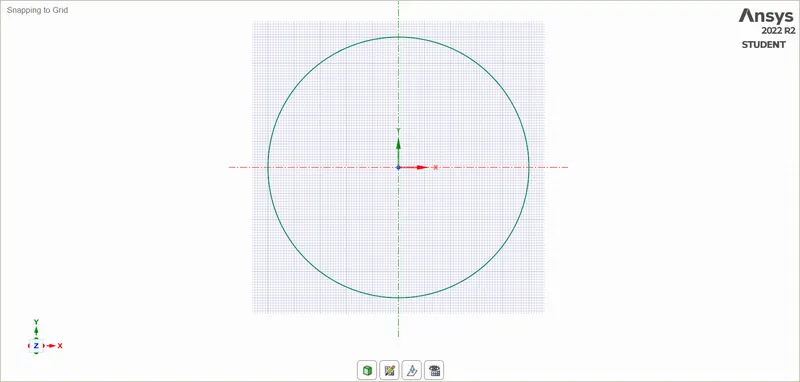
SpaceClaim `->` Select desired Plane by Clickin-on "Select New Sketch Plane" from Graphic Window `->` Click on Sketch Tab `->` Select Circle `->` `ubrace("Select desired location and desired Circle diameter")_("In Our case, Location is Origin and Diameter is 2 meter")` `->` Enter
iii. Steps to Create Computational Domain: -
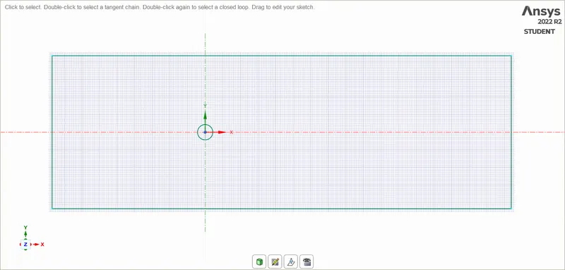
SpaceClaim `->` Click on Sketch Tab `->` Select Rectangle `->` `ubrace("Select desired location and desired Rectangle Dimensions")_("In Our case, Location is (-20,-10) and Dimension are 60X20")` `->` Enter
iv. Steps to Generate the Surface: -
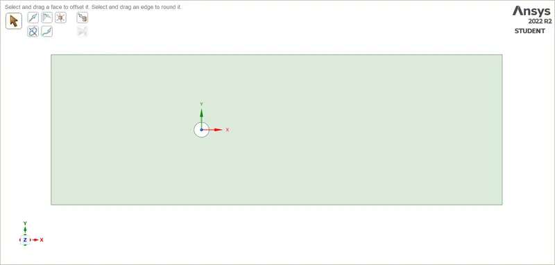
SpaceClaim `->` Select "Return to 3D Mode" from Graphic Window `->` Delete the Unwanted Surface
C. Opening Mechanical(Meshing) and Meshing the Geometry: -
i. Steps to Open Meshing: -
Ansys Workbench `->` Project Schematic `->` Project `->` Mesh `->` Right-Click `->` Edit
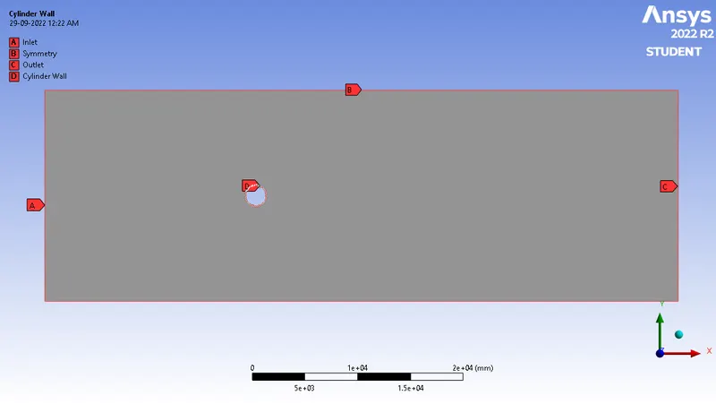
ii. Steps to Name the Boundary: -
Mechanical(Meshing) `->` Model Working Window `->` Select the Boundary `->` Click N `->` Give the desired Name `->` Enter
iii. Steps to Create Triangular Mesh with division at every `10^@` of Cylinder with Inflation Layers: -
a. Mechanical(Meshing) `->` Outline Window `->` Select Mesh `->` Details of Mesh Window `->` Defaults `->` Element Size `->` `ubrace("Give Desired Element Size")_("In our case 500 mm")`
b. Select Mesh `->` Right-Click `->` Select "Method" from Insert `->` Select "Scoping Method" from Scope `->` `ubrace("In Definition Define the desired parameters")_("In our case Select Method as Triangle")`
c. Select Mesh `->` Right-Click `->` Select "Sizing" from Insert `->` `ubrace("Set the desired Parameters")_("In our case, Select Edge and Type as number of Division = 36")`
d. Select Mesh `->` Right-Click `->` Select "Inflation" from Insert `->` `ubrace("Set the desired Parameters")_("In our case, Select geometry and Edge and Inflation Type as First Layer = 5mm and number of the layer as 10")`
e. Select Mesh `->` Right-Click `->` Generate Mesh
D. Opening Ansys Fluent and Performing Analysis: -
i. Steps to Open Ansys Fluent: -
Ansys Workbench `->` Project Schematic `->` Project `->` Setup `->` Right-Click `->` Edit
ii. Steps to Check Mesh: -
Fluent `->` Outline View Window `->` Setup `->` General `->` Mesh `->` Check
iii. Steps to Set up the Physics: -
a. Fluent `->` Physics `->` Models `->` Viscous `->` `ubrace("Select Desired Viscous Model")_("In our case, Laminar")` `->` Enter
iv. Steps to Set up Material, Cell Zone Condition, and Boundary Condition: -
a. Fluent `->` Physics `->` Materials `->` Create/Edit... `->` `ubrace("Select/Create the desired Fluid")_("In our case, Create a User Defined Fluid with density = 1 and Viscosity = 0.05")` `->` Enter
b. Fluent `->` Physics `->` Zone `->` Cell Zone `->` Select the desired Component `->` Edit `->` `ubrace("Make the desired Change")_("In our case, change the fluid to User defined Fluid")` `->` Enter
c. Fluent `->` Physics `->` Zone `->` Boundaries `->` Select the desired Component `->` Select the Desired Type for that Component `->` Edit `->` Add the Values for the Component `->` Apply & Close
v. Steps to Set up Reports: -
Fluent `->` Solution `->` Reports `->` Definition `->` New `->` Select the Desired Report `->` Rename the Report `->` Change the Field Variable to Desired Variable `->` Select the desired Surface `->` Ok
vi. Steps to Run Analysis: -
a. Fluent `->` Solution `->` Initialization `->` Initialize
b. Fluent `->` Solution `->` Run Calculations `->` No. of Iterations `->` Set to desired Iterations
c. Fluent `->` Solution `->` Run Calculations `->` Calculate
Output Generated after Each Step Before Analysis: -
A. Geometry: -
i. Creating Circle: -
ii. Determining Computational Domain and Creating Computational Domain: -
As the Characteristic length of the Cylinder(Diameter) is 2 m. So for the computational Domain taking the inlet length as 10 times the Characteristic Length, the Outlet length as 20 times the Characteristic Length, and the Width as 5 times of Characteristic Length.
Hence,
Inlet Length from Cylinder = 10xD = 20 m
Outlet Length from Cylinder = 20xD = 40m
Width Length from Cylinder = 5xD = 10m
B. Meshing: -
i. After Naming the Boundaries: -
ii. After Meshing: -
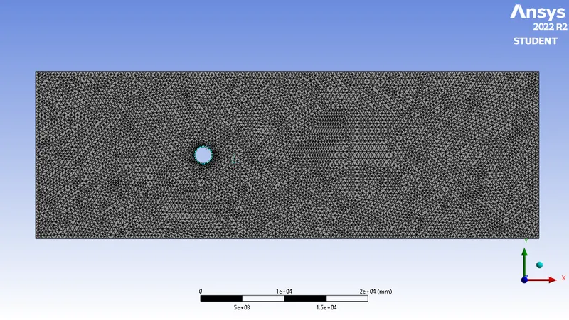
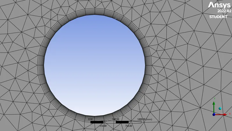
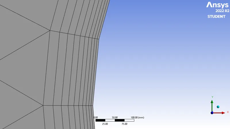
C. Setup: -
i. After Loading in Fluent: -
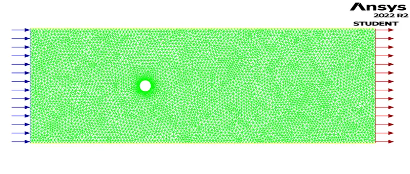
Output/Results Generated after Analysis: -
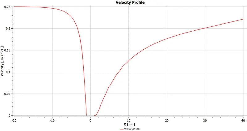
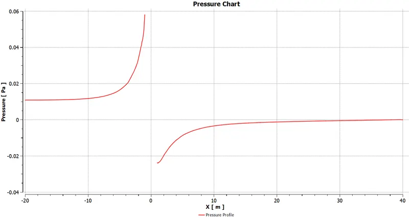
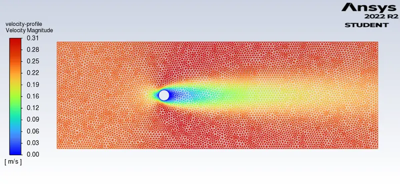
A. Case 1: Reynolds Number = 10`(=> V_("Inlet") = 0.25 "m/s")`
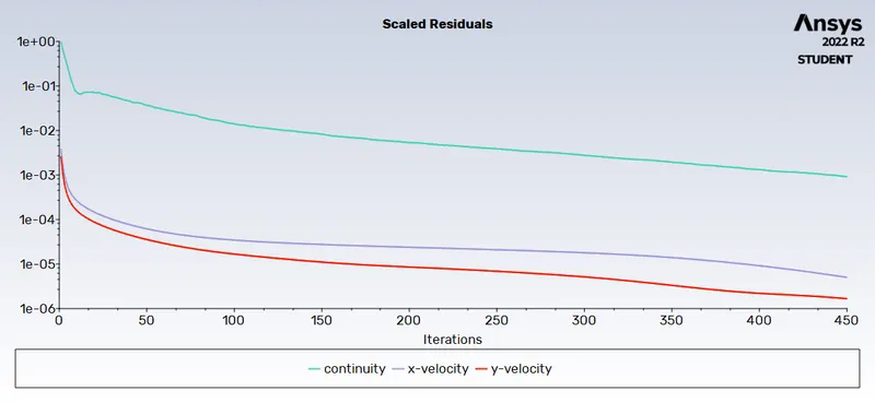
i. Calculations Done while Iterations: -
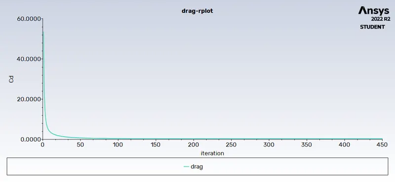
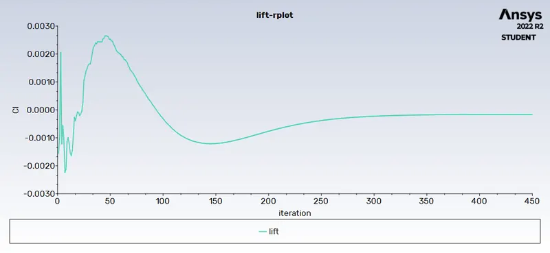
ii. The Drag and Lift experienced by Cylinder: -
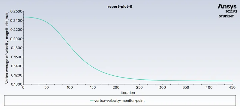
iii. Vortex Velocity Observed at Monitor Point: -
iv. The Velocity and Pressure Chart: -
v. The Velocity Contours: -
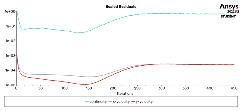
B. Case 2: Reynolds Number = 100`(=> V_("Inlet") = 2.5 "m/s")`
i. Calculations Done while Iterations: -
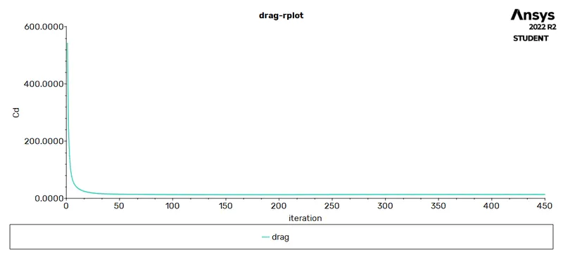
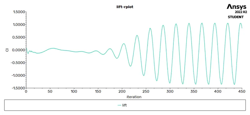
ii. The Drag and Lift experienced by Cylinder: -
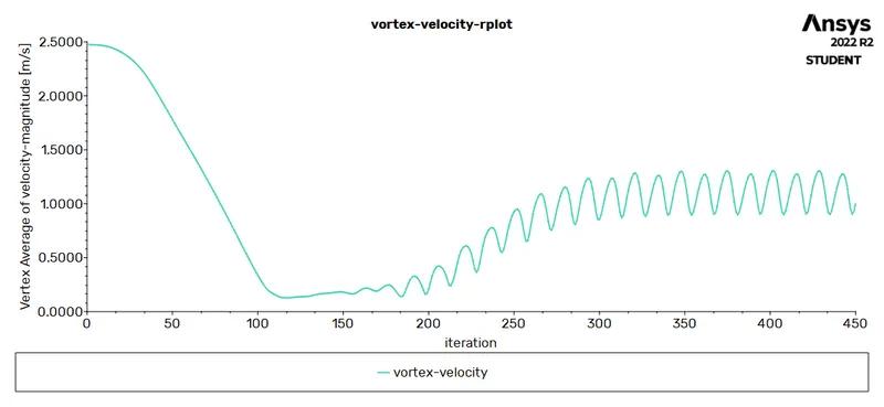
iii. Vortex Velocity Observed at Monitor Point: -
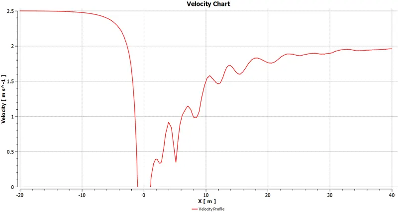
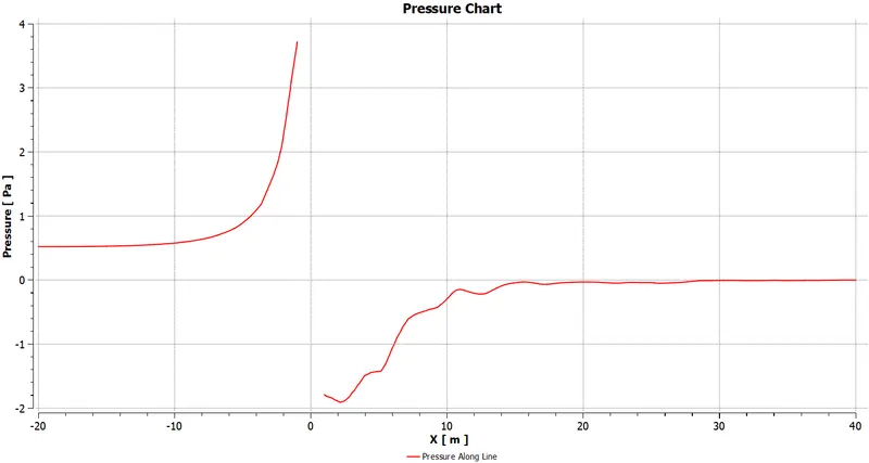
iv. The Velocity and Pressure Chart: -
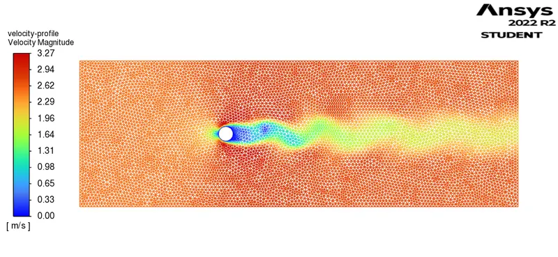
v. The Velocity Contours: -
C. Case 3: Reynolds Number = 1000`(=> V_("Inlet") = 25 "m/s")`
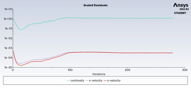
i. Calculations Done while Iterations: -
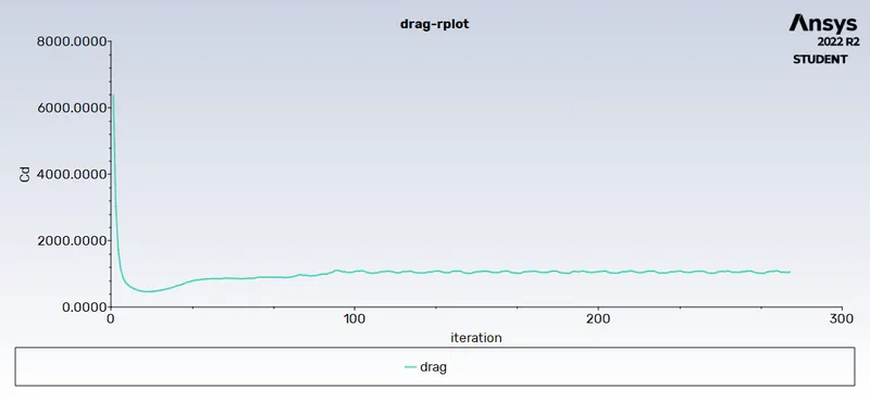
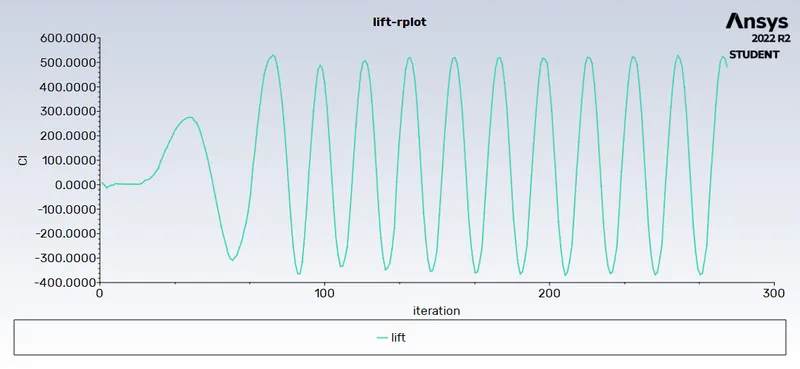
ii. The Drag and Lift experienced by Cylinder: -
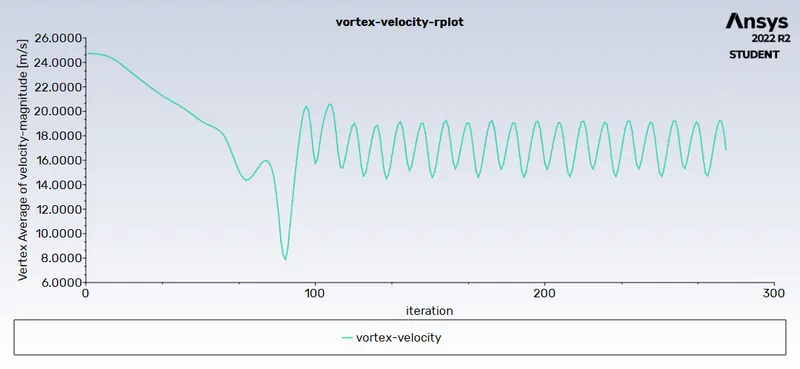
iii. Vortex Velocity Observed at Monitor Point: -
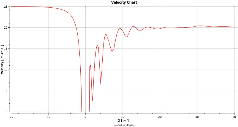
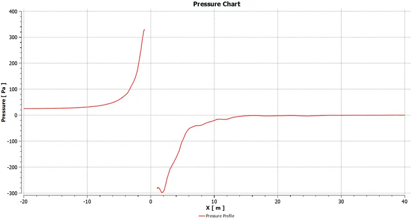
iv. The Velocity and Pressure Chart: -
v. The Velocity Contours: -
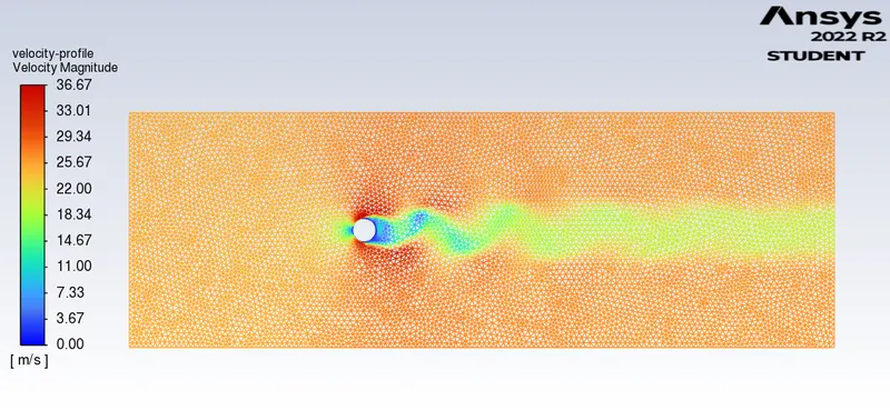
D. Case 4: Reynolds Number = 10000`(=> V_("Inlet") = 250 "m/s")`
i. Calculations Done while Iterations: -
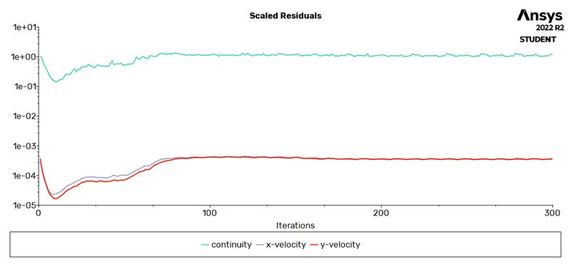
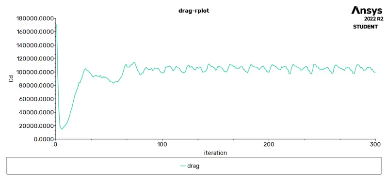
ii. The Drag and Lift experienced by Cylinder: -
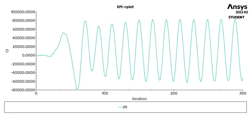
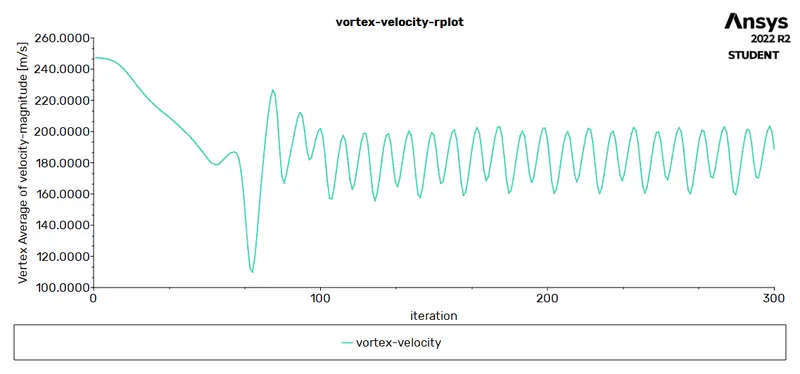
iii. Vortex Velocity Observed at Monitor Point: -
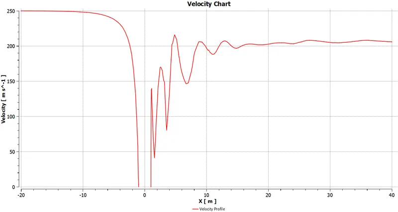
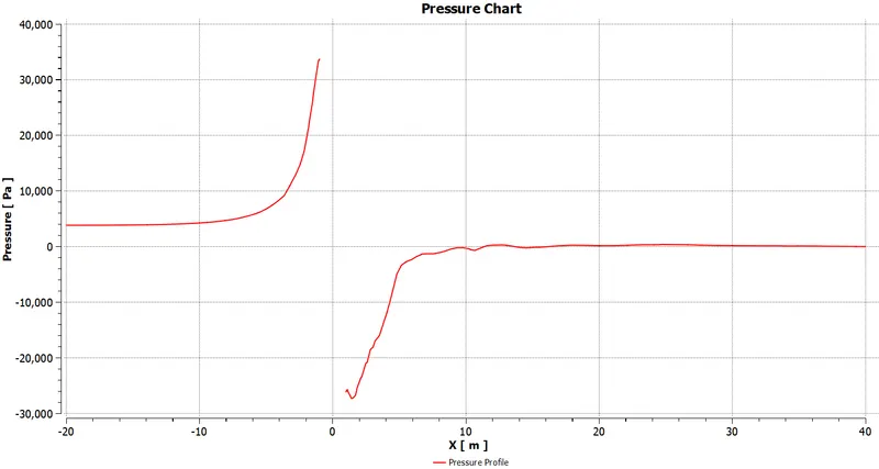
iv. The Velocity and Pressure Chart: -
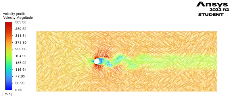
v. The Velocity Contours: -
D. Case 4: Reynolds Number = 100000`(=> V_("Inlet") = 2500 "m/s")`
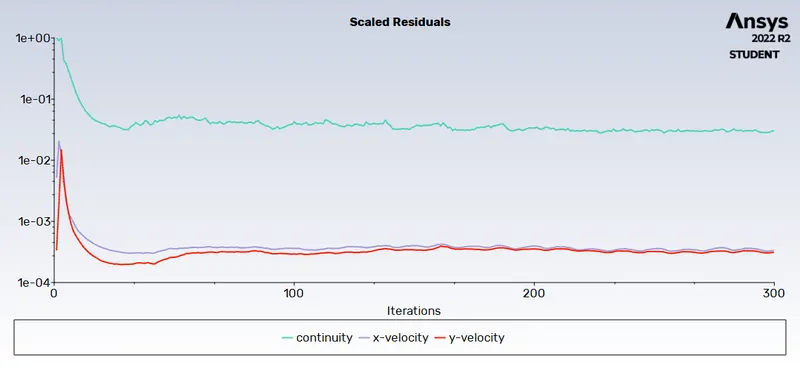
i. Calculations Done while Iterations: -
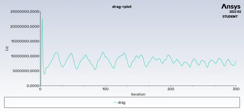
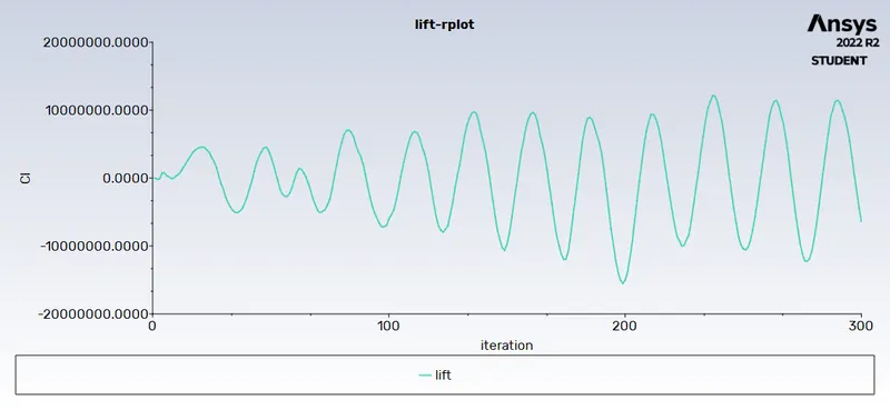
ii. The Drag and Lift experienced by Cylinder: -
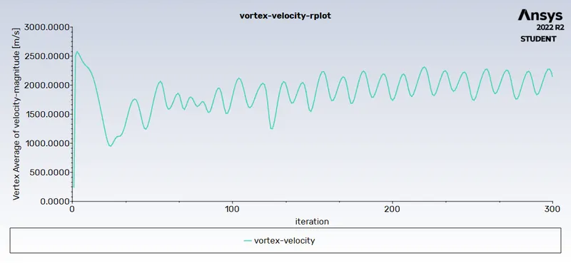
iii. Vortex Velocity Observed at Monitor Point: -
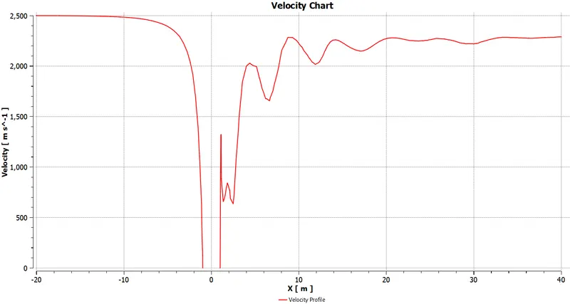
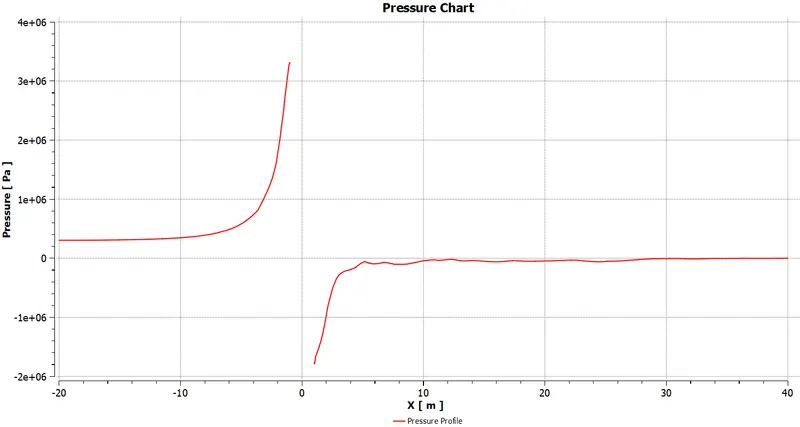
iv. The Velocity and Pressure Chart: -
v. The Velocity Contours: -
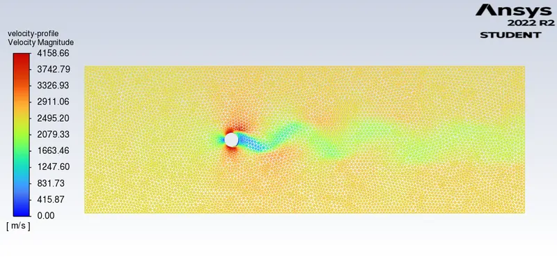
Karman vortex street: -
The Repeating Swirling Vortices are formed due to Vortex Shedding when a fluid flows over a blunt Body and an unsteady flow separation starts to happen. This phenomenon is called Karman Vortex Street.
This phenomenon can be calculated using the Strounhal Number, which is a dimensionless number that describes the oscillating flow mechanism of a body when fluid flows across it.
Method to Calculate Strounhal Number: -
Strounhal Number(St) = `(fL)/u`
where, `f ->` Frequency of Vortex Shedding
`L ->` Characteristic Length of the Blunt Body
`u ->` Fluid Velocity
Calculating Strounhal Number at Reynolds Number = 100: -
For Calculation of Strounhal Number, a Transient State Solution is required and So the Simulation that was done above using a Steady State Solver at Reynolds Number = 100 is done with the same parameters with the difference of using a Transient state Solver.
The Lift Plot generated for the flow over a cylinder using a transient state solver is used to estimate the frequency of oscillation of vortices.
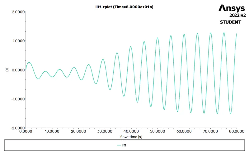
From the above Lift Plot,
Frequency`(f) = 1/5 sec^-1`
And,
As Characteristic Length = 2 m
And Fluid Velocity = 2.5 m/sec
`St = (fL)/u`
`=> St_("(RE = 100)") = 0.16`
| Strounhal Number at Reynolds Number = 100 | 0.16 |