Week 2 - Flow over a Cylinder.

AIM:

Simulate the flow over a cylinder and explain the phenomenon of Karman vortex street.

OBJECTIVES:

1. Simulate the flow with the steady and unsteady case and calculate the Strouhal Number for Re= 100.
2. Calculate the drag and lift coefficient over a cylinder by setting the Reynolds number to 10,100,1000,10000 & 100000.
3. Effect of Reynolds number on the coefficient of drag.
4. Study the vortex shedding behind the cylinder.

THEORY:

Flow over a cylinder is similar to the study of any external flow and its parameters such as lift and drag forces acting on the moving object in a given fluid domain. This helps us determine, overcome or reduce the lift and drag forces acting on the moving object and obtain the maximum efficiency for the moving object. Apart from the lift and drag coefficient, there are many parameters that influence the flow body such as the Reynolds number, dynamic viscosity, and medium of fluid over the body.

Drag is the primary aerodynamic force acting on an object in moving through the fluid. The relationship between the drag and velocity of the surrounding is summarized by the drag coefficient. Hence the flow rate determines the Reynolds number so it's essential to determine the relationship between the drag coefficient and the Reynolds number. Turbulent flow where the Reynolds number is large will create more drag on a moving object compared to laminar flow.

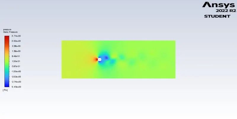
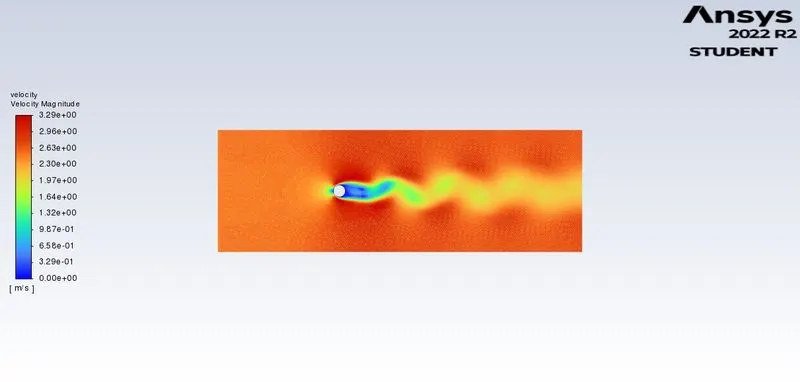
VORTEX SHEDDING is an oscillating flow that occurs when a fluid such as air or water flows past as opposed to streamlining on a body(depending on the size and shape of the body) at a certain velocity. During this flow, vortices are created at the back of the body and detach periodically from either side of the body forming VON KARMAN VORTEX. The fluid flow past the object creates alternating low-pressure vortices on the downstream side of the object.

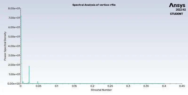
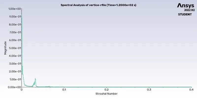
The frequency at which vortex shedding takes place for a cylinder is related to the Strouhal number

`St=(f*D)/V`

Where St is the dimensionless strouhal number, f is the vortex shedding frequency(`s^-1`), D is the diameter of the cylinder (m), and V is the flow velocity(`m*s^-1`). strouhal number depends on the Reynolds number.

Reynolds number for a flow is a measure of the ratio of inertia force to viscous force in the flow of a fluid around a body.

`Re=(U*L)/(nuo)`

U is the flow speed of the fluid, L is the characteristics length of the body, `and nuo`is the kinematic viscosity.

MODELLING AND MESHING USING ANSA:

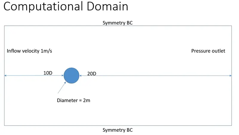
• Initially, I am creating the Cylinder with a 2m diameter at the origin point of the XY plane and the external boundary(computational domain) around the cylinder is designed as shown in the above diagram.
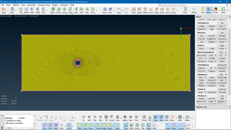
• In the next step, I am creating mesh around the cylinder for various mesh element sizes such as 5m, 4m, and 2.5m(We are looking for 3 different mesh sizes in order to study the accurate result obtained based on which mesh element size ).
• In order to capture the physics around the cylinder, we can create the boundary layers(Inflation layers) based on the Y+ value for the external flow simulation around the cylinder surface.

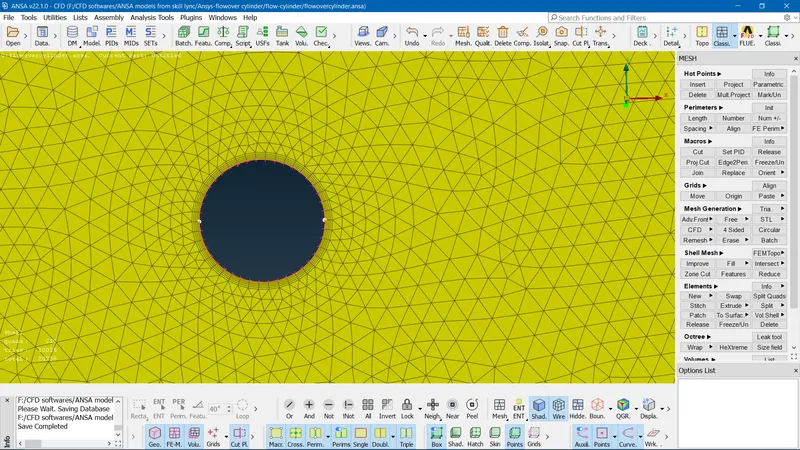
• Since it is a 2D model we cannot create the inlet and outlet hence we have to change the model FLUENT 2D. So that we can assign the boundary layers such as velocity-inlet, pressure-outlet, and symmetry boundary condition.
• Finally, I am exporting the cylinder model from ANSA to .msh format to proceed with solver, and post-processing calculations using ANSYS fluent.

MESHING QUALITY AND PROPERTIES:

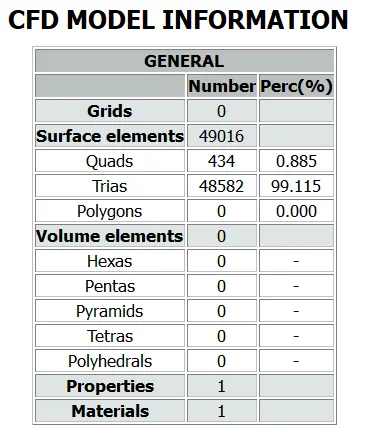
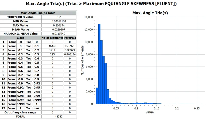
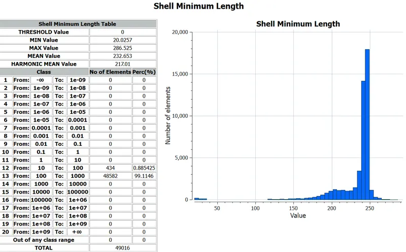
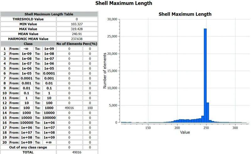
Meshing is performed by referring to the CFD report as shown in the above images obtained from ANSA, we can study that for mesh element size of 2.5m for the boundary conditions. For the cylinder wall, I am considering the mesh element size of 1.8m so that when ADVANCE meshing is done we get varying mesh from boundary to wall surface. Also, I have created 10 inflation layers around the cylinder surface with an inflation layer height of 0.2m. Total surface elements containing TRIA of 49016 elements of 99% and surface quad elements of 434 with 0.885%. Shell minimum and maximum lengths are obtained in the above graph.

SOLVER, POST-PROCESSING ANSYS FLUENT:

SOLVER SETUP:

• First, we open the ANSYS workbench we get blank space, so we create FLUID FLOW fluent on the workbench. Once this is done we get GEOMETRY, MESH, SETUP, SOLUTION, and RESULTS.
• Once we import the .msh file into the SETUP MODEL of the FLUID FLOW fluent on the workbench.
• we open the SETUP MODEL the surface meshed appears as shown below.

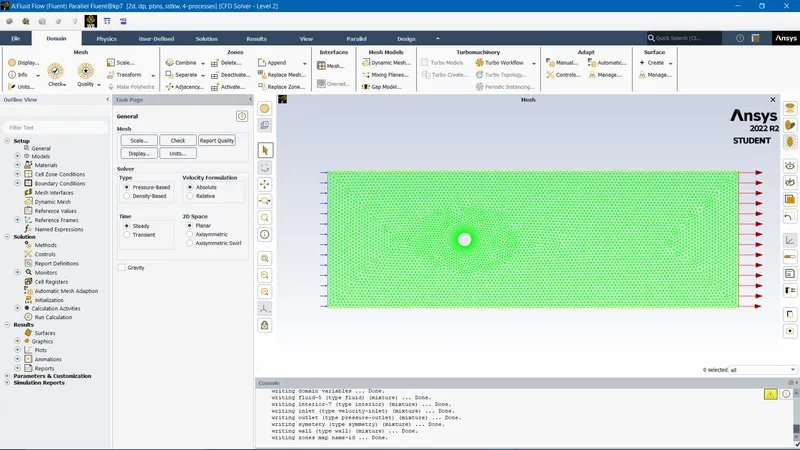
• In this, we provide fundamental physics, types of solver, boundary conditions, and type of turbulent model used.
• Initially, we go for the SOLVER option here we are the type of solver used is PRESSURE BASED SOLVER (M<0.3), and since the variable is not varying with respect to time select the STEADY STATE option also we do study for TRANSIENT STATE option too.
• In the following step in for the PHYSICS, the window selects the VISCOUS option we get the window opened up. Here we are selecting the type of viscous model which is the LAMINAR model(Re<2000) and TURBULENT model (k-epsilon and k-omega SST).
• We are giving the BOUNDARY conditions for the inlet velocity with respect to the Reynolds number that is we are going to calculate the velocity from the Reynolds number formula(i.e Re=10,40,100,1000,10000).
• The wall has a no-slip boundary whereas the top and bottom are in symmetrical boundary conditions.
• The hybrid method is used for initialization.
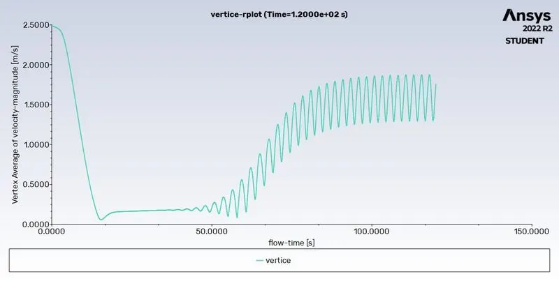
• Monitoring point velocity is the point that is created 10m away from the circle center to monitor the velocity. Also, this helps in calculating the vortex shredding.
• Properties such as user-defined(remain same for every varying in Reynolds number) air properties with a density of `1(kg)/m^3`and viscosity of 0.05 `(Kg)/(m s)`.
• Based on the Reynolds number we are going to study the drag coefficient and lift coefficient.

POST-PROCESSING/RESULTS:

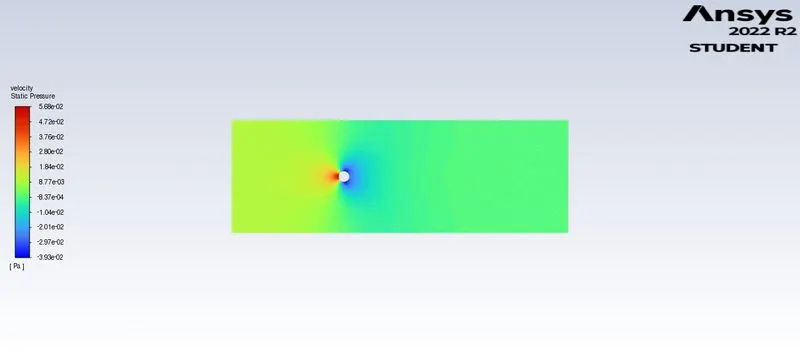
Based on the different Reynolds numbers (10,100,1000,10000,100000) we are going to obtain the contour plots for velocity and pressure(study the drag coefficient and lift coefficient).

For Reynolds number Re-10 STEADY STATE ANALYSIS

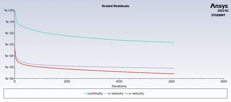
Convergence plot

Lift plot

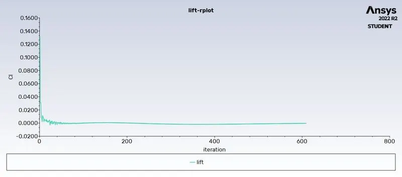
As we can observe below plot the lift coefficient has converged and reached a steady state and the value of the lift coefficient is -0.00039.

Drag plot

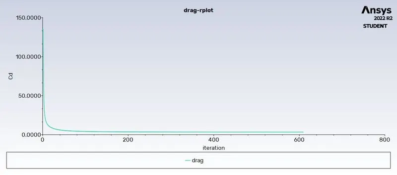
As we can observe below the plot the drag coefficient has converged and reached a steady state and the value of the drag coefficient is 3.34.

Pressure contour

Velocity contour

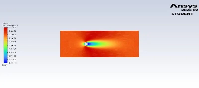
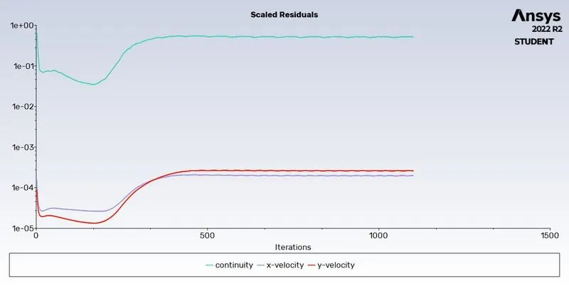
For Reynolds number Re-100 STEADY STATE ANALYSIS

Convergence plot

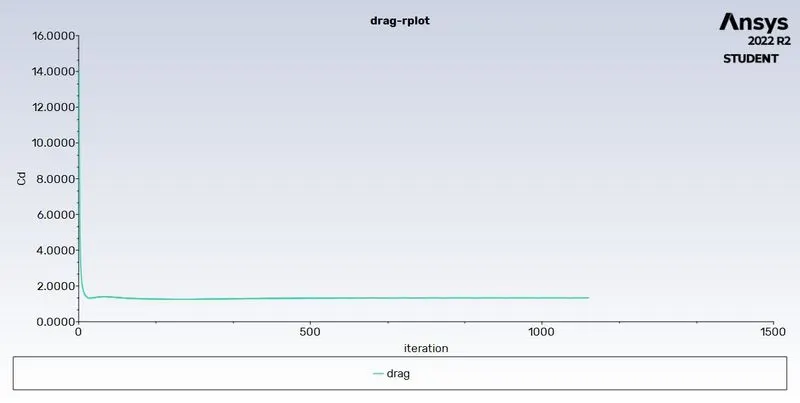
Drag plot

As we can observe below the plot the drag coefficient has converged and reached a steady state and the value of the drag coefficient is 1.33.

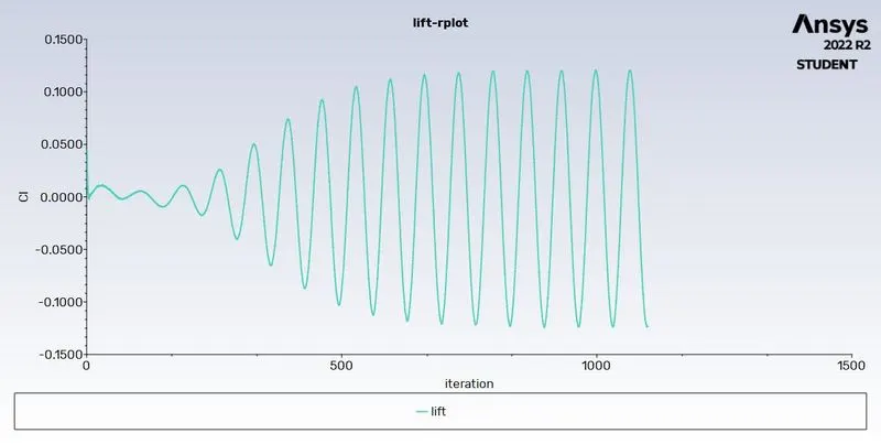
Lift plot

As we can observe below plot the lift coefficient has converged and reached a steady state and the value of the lift coefficient is -0.123.

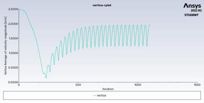
Average velocity magnitude plot

Strouhal number plot

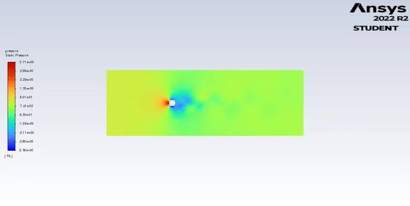
Pressure contour

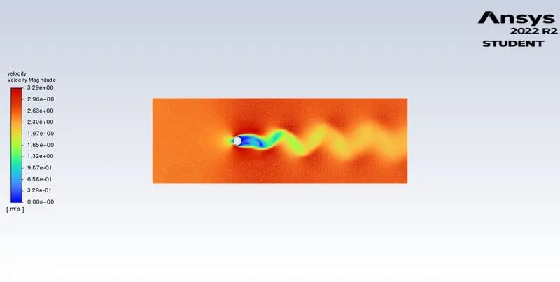
Velocity contour

In the below velocity plot we can see the vortex shedding behind the cylinder.

For Reynolds number Re-100 TRANSIENT STATE ANALYSIS

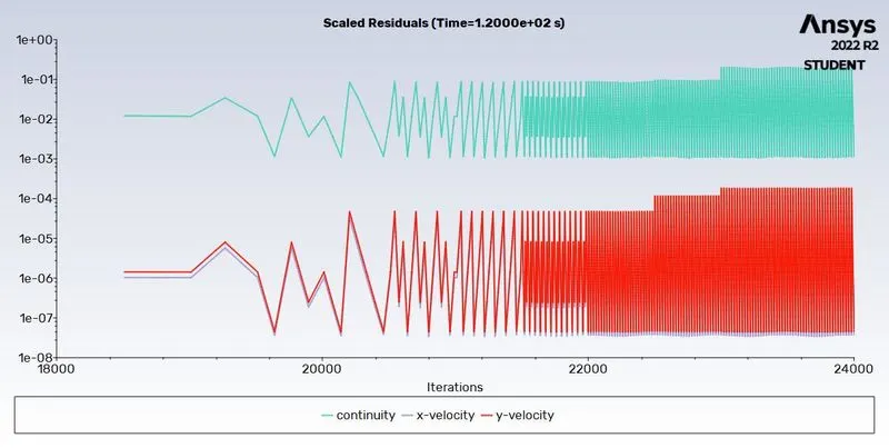
Convergence plot

Drag plot

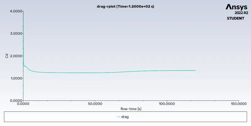
As we can observe below the plot the drag coefficient has converged and reached a steady state and the value of the drag coefficient is 1.44.

Lift plot

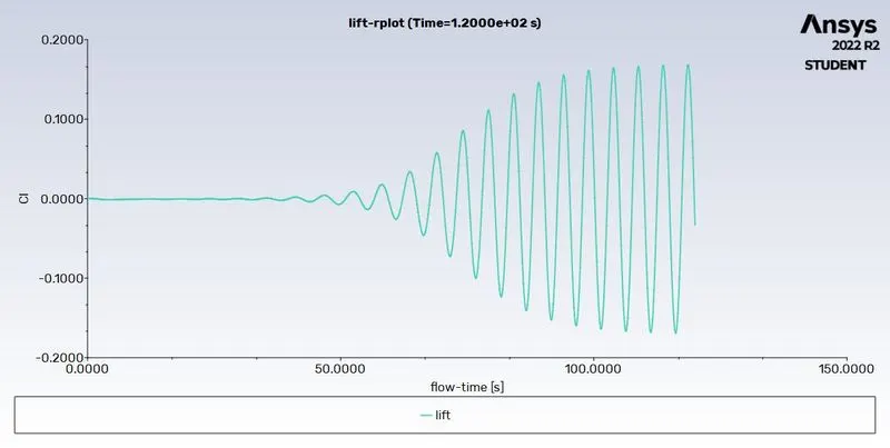
As we can observe below plot the lift coefficient has converged and reached a steady state and the value of the lift coefficient is -0.033.

Average velocity magnitude plot

Strouhal number plot

Pressure contour

Velocity contour

In the below velocity plot we can see the vortex shedding behind the cylinder.

For Reynolds number Re-1000 STEADY STATE ANALYSIS

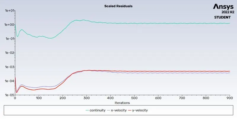
Convergence plot

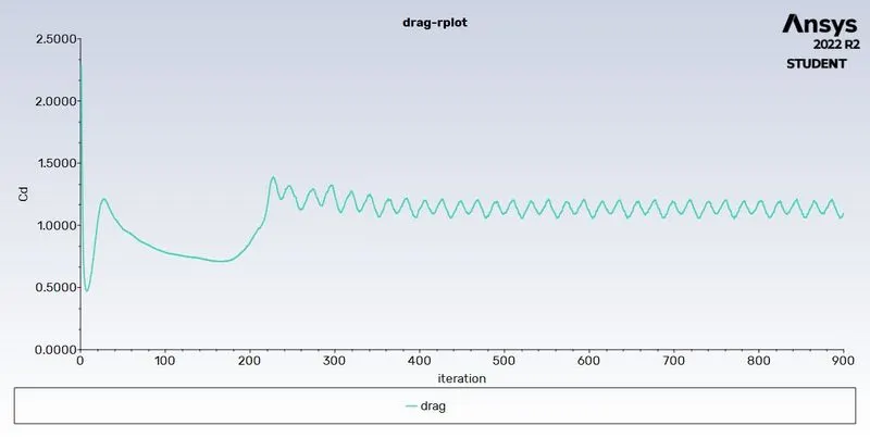
Drag plot

As we can observe below the plot the drag coefficient has converged and reached a steady state and the value of the drag coefficient is 1.21.

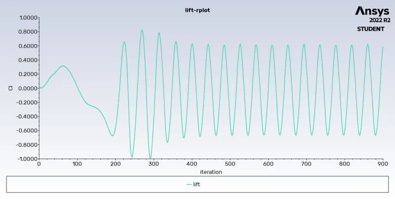
Lift plot

As we can observe below plot the lift coefficient has converged and reached a steady state and the value of the lift coefficient is 0.588.

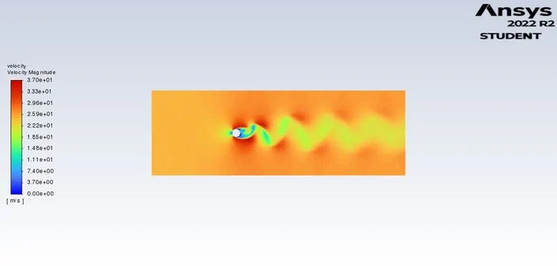
Velocity contour

In the below velocity plot we can see the vortex shedding behind the cylinder.

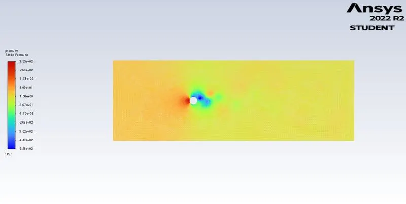
Pressure contour

For Reynolds number Re-10000 STEADY STATE ANALYSIS

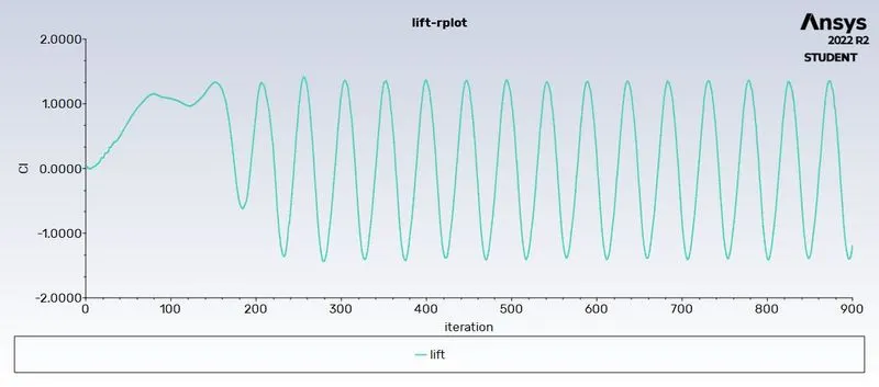
Lift plot

As we can observe below the plot the lift coefficient has converged and reached a steady state and the value of the lift coefficient is 1.09.

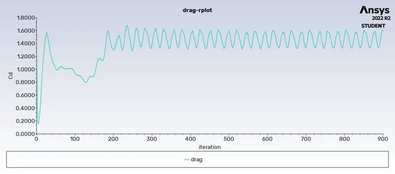
Drag plot

As we can observe below the plot the drag coefficient has converged and reached a steady state and the value of the drag coefficient is 1.05.

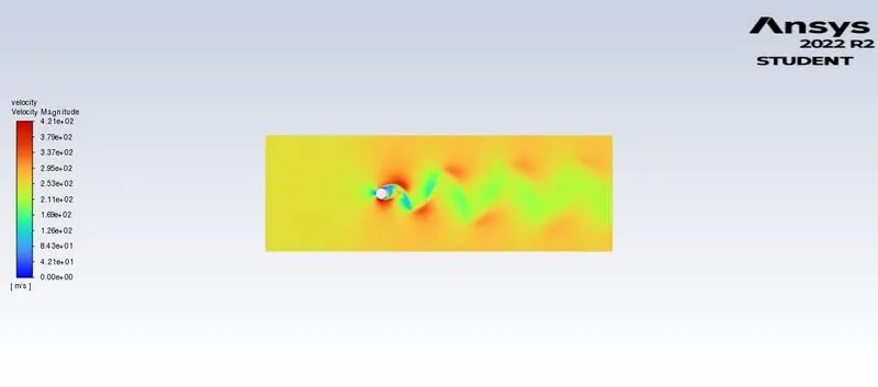
Velocity contour

In the below velocity plot we can see the vortex shedding behind the cylinder.

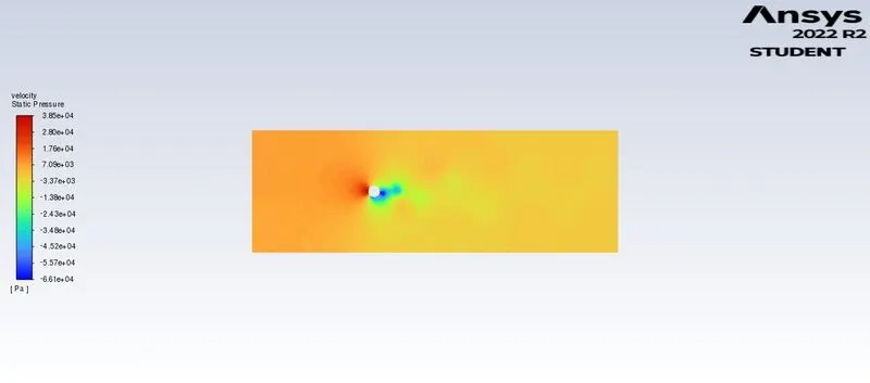
Pressure contour

For Reynolds number Re-100000 STEADY STATE ANALYSIS

Drag plot

As we can observe below the plot the drag coefficient has converged and reached a steady state and the value of the drag coefficient is 0.96.

Lift plot

As we can observe below the plot the lift coefficient has converged and reached a steady state and the value of the lift coefficient is 1.049.

Velocity contour

In the below velocity plot we can see the vortex shedding behind the cylinder.

Pressure contour

EFFECT OF REYNOLDS NUMBER ON DRAG COEFFICIENT

• RE =10 illustrates what actually occurs for low velocity. A stable pair of vortices are formed on the downwind side of the cylinder. The flow is separated but steady and the vortices generate a high drag on the cylinder.
• RE = 100 shows the flow as velocity is increased. The downstream vortices become unstable, separate from the body, and are alternately downstream. The wake is very wide and generates a large amount of drag. The alternate shedding is called the Karman vortex street.
• RE = 1000 and 10000 show the flow as the velocity increases even more. The periodic flow breaks down into a chaotic wake. The flow in the boundary layer on the windward side of the cylinder is laminar and orderly and the chaotic wake is initiated. The wake is not quite as wide as for RE =100, so the drag is slightly less.
• RE = 100000 shows the flow at an even higher velocity. The boundary layer transitions to chaotic turbulent flow with vortices of many different scales being shed in a turbulent wake from the body. The separation point is initially slightly downstream from the laminar separation point, so the wake is initially slightly smaller and the drag is less than the corresponding laminar drag.

REFERENCES

1. B.N. Rajani, A. Kandasamy, Sekhar Majumdar, Numerical simulation of laminar flow past a circular cylinder, Applied Mathematical Modelling, Volume 33, Issue 3, 2009,https://doi.org/10.1016/j.apm.2008.01.017.