Week 2 - Flow over a Cylinder.
AIM:
To Understand and Simulating the Steady and Transient Flow over a Cylinder in Ansys Fluent and observe the variation of velocity and pressure in a domain for different Reynolds Numbers.
Simulating the flow over a cylinder and to explain the phenomenon of Karman vortex street.
INTRODUCTION:
Flow over a cylinder is a classical problem for understanding the flow over an obstacle. The geometry of the cylinder is simple and allows us to understand all the complexities that occur and turbulence for different Reynolds Numbers. Reynolds Number helps us to understand the flow patterns of the different fluid flow situations. The different range of Reynolds Numbers represents different flow patterns. At low Reynolds Numbers, the flow pattern is observed to be Laminar i.e., Smooth, Constant fluid motion. At higher Reynolds Numbers the flow pattern is observed to be Turbulent i.e., Chaotic eddies, Vortices, and Flow instabilities. In this project, we will try to understand the variation of velocity and pressure in certain flow directions for different Reynolds Numbers by simulating it with proper boundary conditions, Mesh sizing, Convergence criteria using Ansys Fluent Simulation.
THEORY:
In fluid dynamics, a Karman vortex street (or a von Kármán vortex street) is a repeating pattern of swirling vortices, caused by a process known as vortex shedding, which is responsible for the unsteady separation of flow of a fluid around blunt bodies.
It is named after the engineer and fluid dynamicist Theodore von Kármán and is responsible for such phenomena as the "singing" of suspended telephone or power lines and the vibration of a car antenna at certain speeds.
A vortex street will form only at a certain range of flow velocities, specified by a range of Reynolds numbers (Re), typically above a limiting Re value of about 90. The (global) Reynolds number for a flow is a measure of the ratio of inertial to viscous forces in the flow of a fluid around a body or in a channel, and may be defined as Reynold's Number.
Reynolds Number: It is defined as the ratio of inertial forces to viscous forces within the fluid which is subjected to relative internal movement due to different fluid velocities. The region where these forces change behavior is known Boundary layer. This relative movement generates fluid friction, which is a factor in developing turbulent flow. Counteracting this effect is the viscosity of the fluid, which tends to inhibit turbulence. The Reynolds number quantifies the relative importance of these two types of forces for given flow conditions and is a guide to when the turbulent flow will occur in a particular situation. This ability to predict the onset of turbulent flow is an important design tool for equipment such as piping systems and aircraft wing.
With respect to laminar and turbulent flow regimes:
- laminar flow occurs at low Reynolds numbers, where viscous forces are dominant, and is characterized by smooth, constant fluid motion;
- turbulent flow occurs at high Reynolds numbers and is dominated by inertial forces, which tend to produce chaotic eddies, vortices, and other flow instabilities.
Mathematically Reynolds Number is defined as:
`Re= (rhov D)/mu`=`(vD)/nu`
`rho`- Density of the fluid
v-Velocity of the fluid
D-Diameter of the tube or cylinder
`nu`-Kinematic viscosity
`mu`-Dynamic viscosity
Strouhal Number:
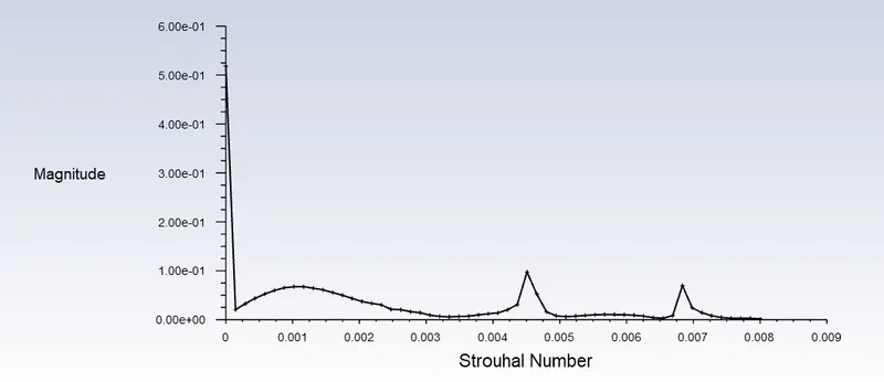
In dimensional analysis, the Strouhal number (St, or sometimes Sr to avoid the conflict with the Stanton number) is a dimensionless number describing oscillating flow mechanisms. The parameter is named after Vincent Strouhal, a Czech physicist who experimented in 1878 with wires experiencing vortex shedding and singing in the wind. The Strouhal number is an integral part of the fundamentals of fluid mechanics.
The Strouhal number is often given as

where f is the frequency of vortex shedding, L is the characteristic length (for example, hydraulic diameter or the airfoil thickness) and U is the flow velocity.
There are some concepts to be discussed, they are
Boundary-Layer:
A boundary layer is the layer of fluid in the immediate vicinity of a bounding surface where the effects of viscosity are significant.
The viscous nature of airflow reduces the local velocities on a surface and is responsible for skin friction. The layer of air over the wing's surface that is slowed down or stopped by viscosity, is the boundary layer. There are two different types of boundary layer flow: laminar and turbulent.
Laminar boundary layer flow
The laminar boundary is a very smooth flow, while the turbulent boundary layer contains swirls or "eddies." The laminar flow creates less skin friction drag than the turbulent flow but is less stable. Boundary layer flow over a wing surface begins as a smooth laminar flow. As the flow continues back from the leading edge, the laminar boundary layer increases in thickness.
Turbulent boundary layer flow
At some distance back from the leading edge, the smooth laminar flow breaks down and transitions to a turbulent flow. From a drag standpoint, it is advisable to have the transition from laminar to turbulent flow as far aft on the wing as possible or have a large amount of the wing surface within the laminar portion of the boundary layer. The low energy laminar flow, however, tends to break down more suddenly than the turbulent layer.
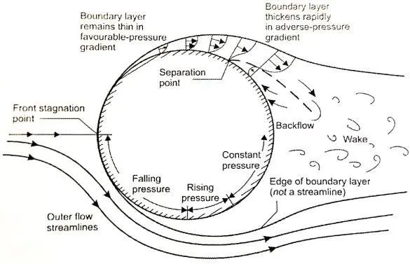
Flow separation:
It is important to understand when and why the flow separates when fluid flows through the obstacle or cylinder in this case. In boundary-layer, due to viscosity, there is a change in pressure along the surface of the body. This causes the boundary layer to be sensitive to the pressure gradient (as the form of a pressure force acting upon fluid particles). If the pressure decreases in the direction of the flow, the pressure gradient is said to be favorable. In this case, the pressure force can assist the fluid movement and there is no flow retardation. However, if the pressure is increasing in the direction of the flow, an adverse pressure gradient condition as so it is called exist. In addition to the presence of a strong viscous force, the fluid particles now have to move against the increasing pressure force. Therefore, the fluid particles could be stopped or reversed, causing the neighboring particles to move away from the surface. This phenomenon is called the boundary layer separation or flow separation.
Wake:
Consider a fluid particle flows within the boundary layer around the circular cylinder. From the pressure distribution measured in an earlier experiment, the pressure is a maximum at the stagnation point and gradually decreases along the front half of the cylinder. The flow stays attached in this favorable pressure region as expected. However, the pressure starts to increase in the rear half of the cylinder and the particle now experiences an adverse pressure gradient. Consequently, the flow separates from the surface and creating a highly turbulent region behind the cylinder called the wake. The pressure inside the wake region remains low as the flow separates and a net pressure force (pressure drag) is produced.
SIMULATION SETUP:
CAD Design is done using Spaceclaim --> Meshing using Ansys mesh --> Simulation using Fluent
Before starting the simulation we need to prepare a solid cylinder by making a sketch and using pull to surface it to a certain length in sketch tab in Spaceclaim .
Geometry:
2D CAD of solid cylinder of 2m radius inside a rectangular domain of length 60*20m is prepared. 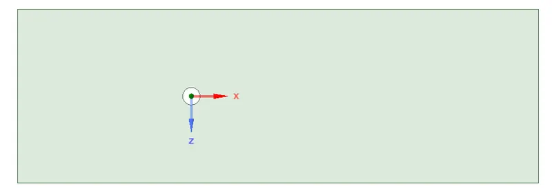
MESH
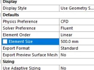
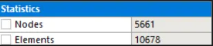
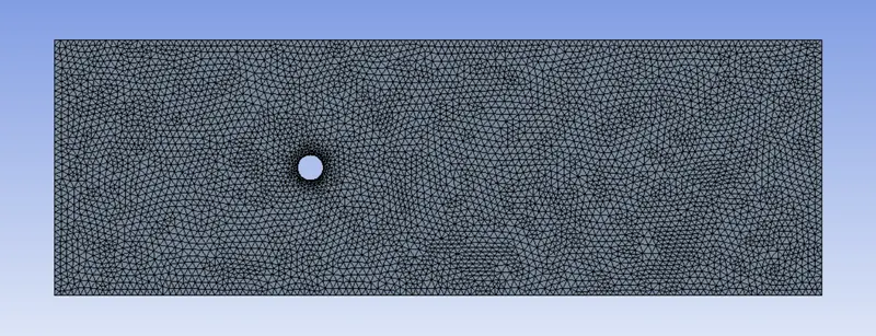
Mesh method: all triangles
number of division about the edge of the cylinder: 36

Inflation layer :
FLT=5mm
growth rate =1.2
no of layers=8
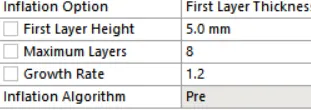
inflation Layer and the number of divisions are used to capture the circular geometry so that nodes can calculate values.
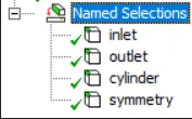 Boundaries are named as in fig
Mesh O/P:
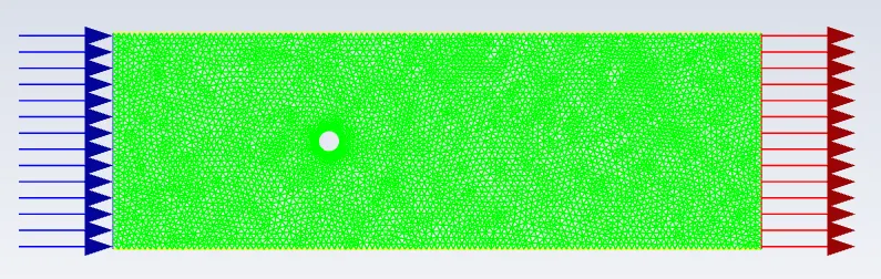
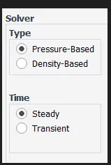
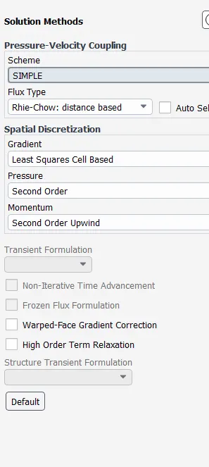
FLUENT SETUP DETAILS
MATERIAL SPECIFICATION:
air with density =1 and mu = 0.05
VISCOUS MODEL
Laminar
BOUNDARY CONDITIONS
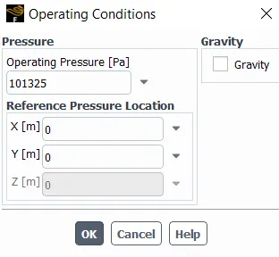
Outlet as pressure-outlet
no slip condition for wall
and 0 gauge pressure for the outlet as operating conditions are set to 1atm.
Result:
PART-I
- Simulating the flow with the steady and unsteady(transient) case and calculate the Strouhal Number for Re= 100
Reynolds Number = 100
The simulation in which we , use the Reynolds Number formula to calculate the Inlet Velocity of the airflow is ,
`Re = (rho.u.L)/mu`
100 = (1) (u) (2) / (0.05)
u = 2.5 m/s
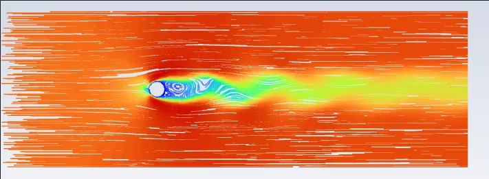
a) Steady :
* velocity contour to show vortex shedding behind the cylinder.
* Plots of the coefficient of drag and lift:
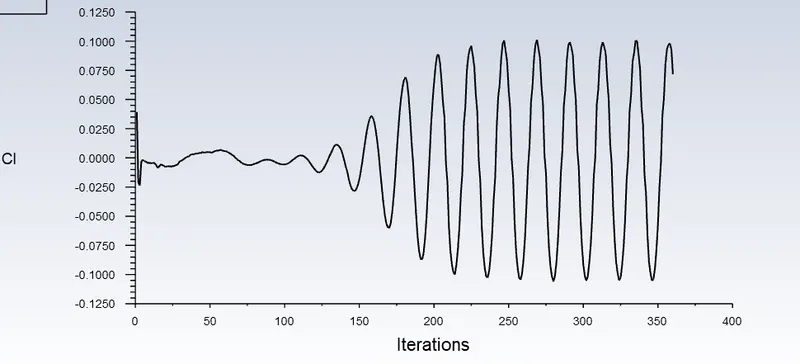
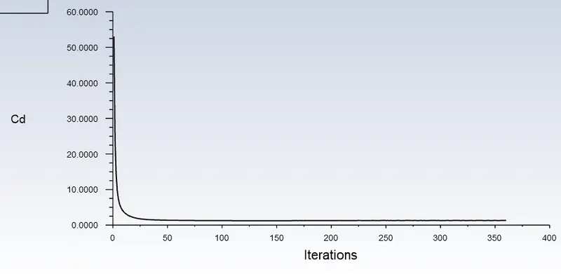
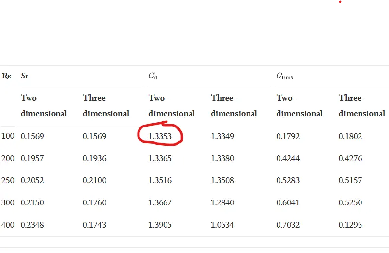
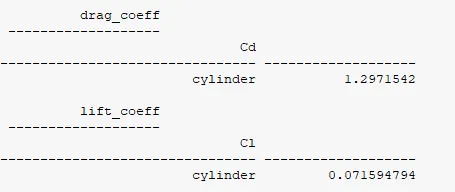
Drag Coefficient when compared to the experiment result from Reference paper.
Cd in Ref paper = 1.3353 , computational Cd = 1.2971
error% = (approx - expected) / expected = (1.2971 - 1.3353) / 1.3353 = 2.8% error
* Hence Results is validated with literature and error is less than 5 %
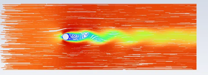
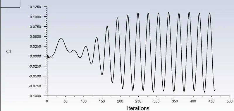
b) Transient:(Re = 100)
* velocity contour to show vortex shedding behind the cylinder.
* Plots of the coefficient of drag and lift:
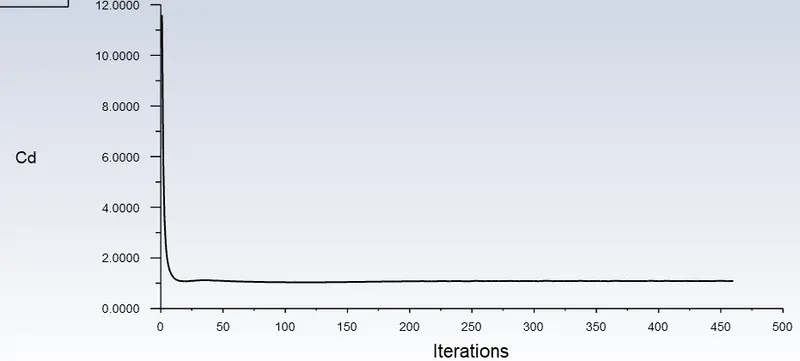
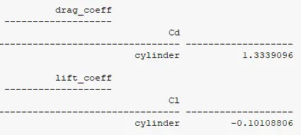
Drag Coefficient when compared to the experiment result from Reference paper.
Cd in Ref paper = 1.3353 , computational Cd = 1.3339
error% = (approx - expected) / expected = (1.3339 - 1.3353) / 1.3353 .... there is not much error to calculate
* Hence Results is validated with literature and error is less than 5 %
Strouhal number:
PART-II
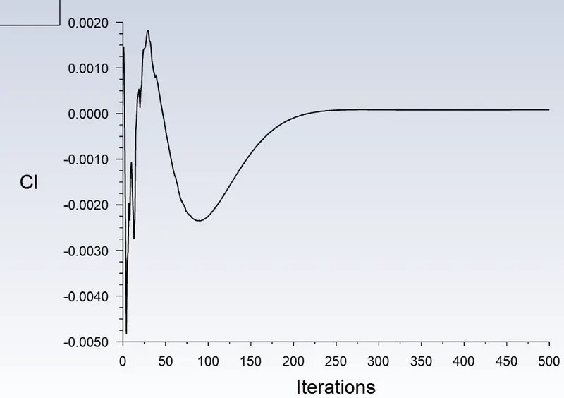
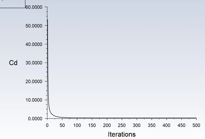
- Calculating the coefficient of drag and lift over a cylinder by setting the Reynolds number to 10,100,1000,10000 & 100000. ( with steady solver)
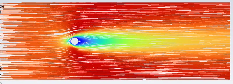
Reynolds Number = 10
The simulation in which we , use the Reynolds Number formula to calculate the Inlet Velocity of the airflow is ,
`Re = (rho.u.L)/mu`
10 = (1) (u) (2) / (0.05)
u = 0.25 m/s
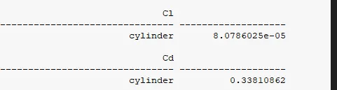
* velocity contour to show vortex shedding behind the cylinder.
* Plots of the coefficient of drag and lift:
Reynolds Number = 1000
The simulation in which we , use the Reynolds Number formula to calculate the Inlet Velocity of the airflow is ,
`Re = (rho.u.L)/mu`
1000 = (1) (u) (2) / (0.05)
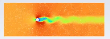
u = 25 m/s
* velocity contour to show vortex shedding behind the cylinder.
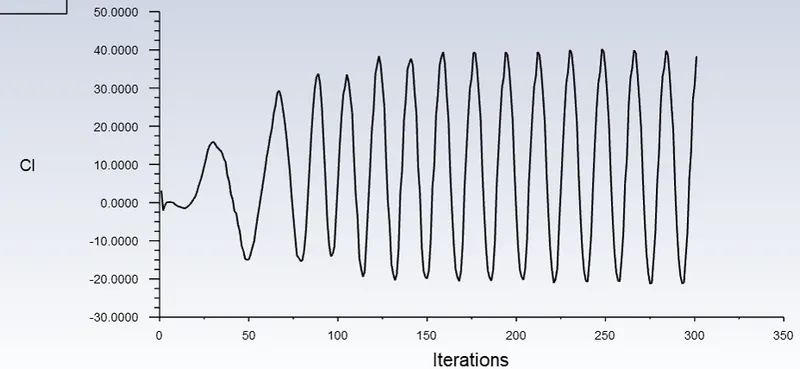
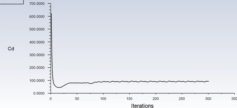
* Plots of the coefficient of drag and lift:
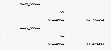
Reynolds Number = 10000
The simulation in which we , use the Reynolds Number formula to calculate the Inlet Velocity of the airflow is ,
`Re = (rho.u.L)/mu`
10000 = (1) (u) (2) / (0.05)
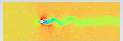
u = 250 m/s
* velocity contour to show vortex shedding behind the cylinder.
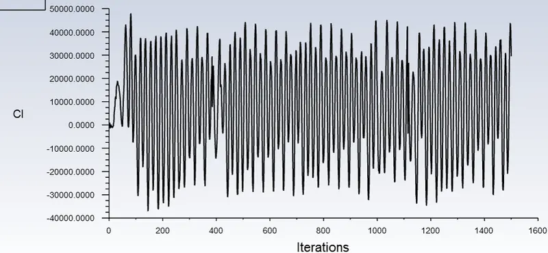
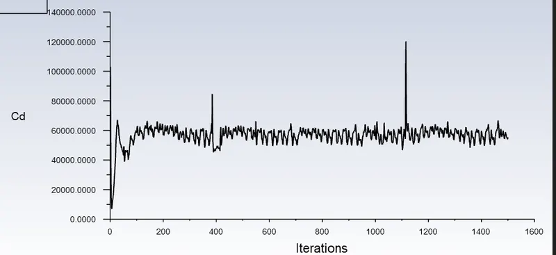
* Plots of the coefficient of drag and lift:
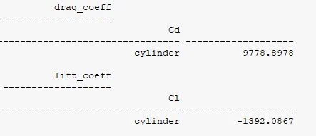
Reynolds Number = 100000
The simulation in which we , use the Reynolds Number formula to calculate the Inlet Velocity of the airflow is ,
`Re = (rho.u.L)/mu`
100000 = (1) (u) (2) / (0.05)
u = 2500 m/s
* velocity contour to show vortex shedding behind the cylinder.
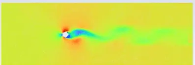
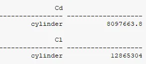
* Plots of the coefficient of drag and lift:
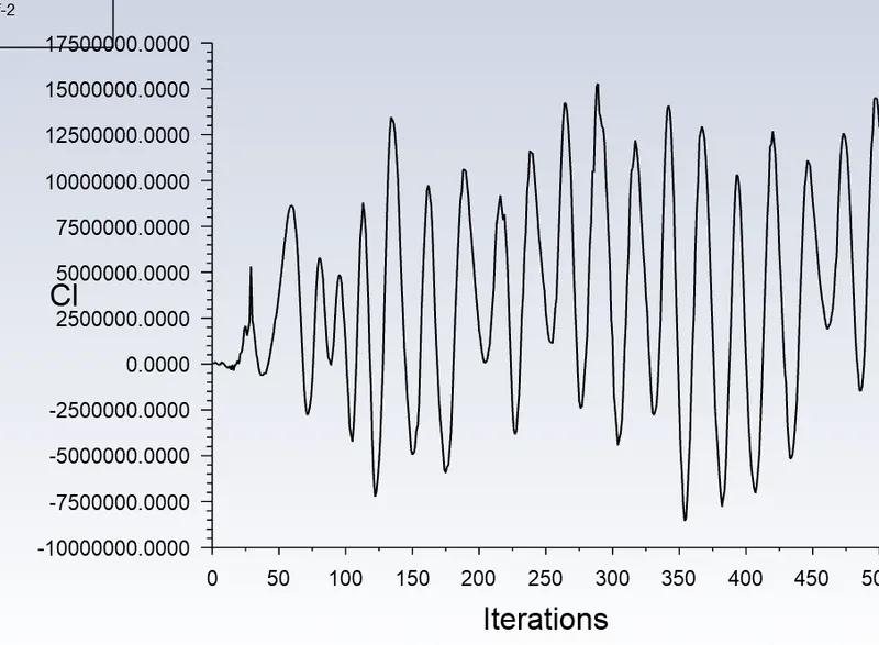
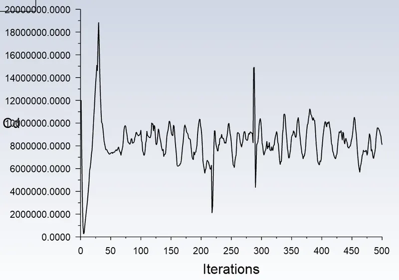
* Validating Results:
Reynolds Number = 100
The simulation in which we , use the Reynolds Number formula to calculate the Inlet Velocity of the airflow is ,
`Re = (rho.u.L)/mu`
100 = (1) (u) (2) / (0.05)
u = 2.5 m/s
a) Steady :
Drag Coefficient when compared to the experiment result from Reference paper.
Cd in Ref paper = 1.3353 , computational Cd = 1.2971
error% = (approx - expected) / expected = (1.2971 - 1.3353) / 1.3353 = 2.8% error
* Hence Results is validated with literature and error is less than 5 %
b) Transient:(Re = 100)
Drag Coefficient when compared to the experiment result from Reference paper.
Cd in Ref paper = 1.3353 , computational Cd = 1.3339
error% = (approx - expected) / expected = (1.3339 - 1.3353) / 1.3353 .... there is not much error to calculate
* Hence Results is validated with literature and error is less than 5 %