Week 2 - Flow over a Cylinder.

Week 2 - Flow over a Cylinder

Aim and Objective:

1. To simulate the flow over a cylinder and explain the phenomenon of Karman vortex street.
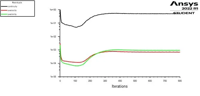
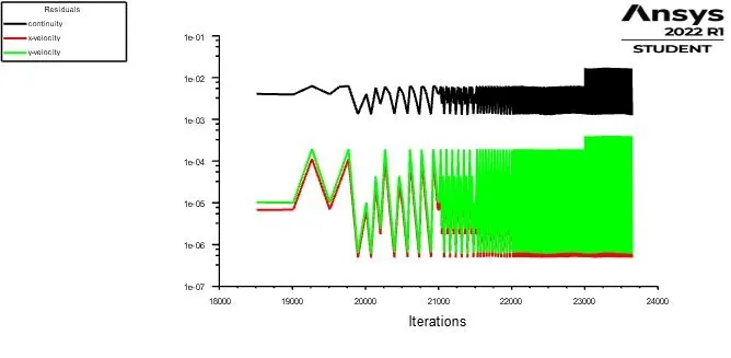
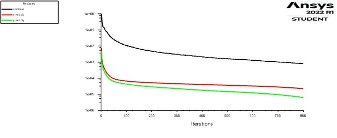
2. To show that the flow has converged.
3. To plot the coefficient of drag and lift.
4. To plot the vortex shedding behind the cylinder.
5. To mention the referred material.

PART-I

1. To simulate the flow with the steady and unsteady case and calculate the Strouhal Number for Re= 100.

PART-II

1. To calculate the coefficient of drag and lift over a cylinder by setting the Reynolds number to 10,100,1000,10000 & 100000. (Run with steady solver)
2. To discuss the effect of Reynolds number on the coefficient of drag.

NOTE:

1. Vary the velocity of the flow to change the Reynolds number.
2. Setting the reference values in Fluent is necessary to get the correct values of drag and lift.

Introduction:

With respect to the extensive experimental and numerical studies almost over a century, flow around a circular cylinder still remains a challenging problem in fluid mechanics, where intensive investigations are continued even today to understand the complex unsteady dynamics of the cylinder wake flow.

Regarding experimental measurements and numerical computations have confirmed the onset of instability of the wake flow behind a cylinder beyond a critical Reynolds number, leading finally to a kind of periodic flow identified by definite frequencies, well-known in the literature as the Von Karman vortex street.

Karman vortex street

In fluid dynamics, a Karman vortex street is a repeating pattern of swirling vortices, caused by a process known as vortex shedding, which is responsible for the unsteady separation of flow of a fluid around blunt bodies.

A vortex street will form only at a certain range of flow velocities, specified by a range of Reynolds numbers (Re), typically above a limiting Re value of about 90. The (global) Reynolds number for a flow is a measure of the ratio of inertial to viscous forces in the flow of a fluid around a body or in a channel and may be defined as a nondimensional parameter of the global speed of the whole fluid flow.

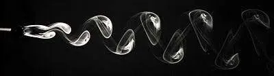
The following table enlists the flow patterns for flow with different Reynolds Number over a circular cylinder.

Reynolds number:

It is the ratio of inertial forces to viscous forces. The Reynolds number is a dimensionless number used to categorize the fluids systems in which the effect of viscosity is important in controlling the velocities or the flow pattern of a fluid and also determine whether a fluid is in laminar or turbulent flow. it is mathematically defined as,

`Re=(rho*V*D)/mu`

In this equation,

`rho = Density`

`V = Velocity`

D = Length of the cylinder

`mu` = Kinematic Viscosity

Coefficient of drag

In fluid dynamics, the drag coefficient is a dimensionless quantity that is used to quantify the drag or resistance of an object in a fluid environment, such as air or water. It is used in the drag equation in which a lower drag coefficient indicates the object will have less aerodynamic or hydrodynamic drag. The drag coefficient is always associated with a particular surface area.

The drag coefficient is represented as,

`C_D = (2F_D)/(rhoU^2A)`

Where F_d is the drag force

ρ is the mass density of fluid

U is the flow speed

A is the reference area

The drag coefficient of any object comprises the effects of the two basic contributors to fluid dynamic drag: skin friction and form drag.

Coefficient of lift

The lift coefficient is a dimensional coefficient that relates the lift generated by a lifting body to the fluid density around the body, the fluid velocity and an associated reference area. A lifting body is a foil or a complete foil bearing body such as a fixed – wing aircraft. Coefficient of lift is a function of the angle of the body to the flow, its Reynolds number and it’s Mach number.

Mathematically it is represented as,

`C_L=(2L)/(rhoU^2A)`

Where L is the lift force

A is the relevant surface area

ρ is the fluid density

u is the flow speed

Strouhal number:

The Strouhal number is a dimensionless value useful for analysing oscillating unsteady fluid flow dynamics problems.

Mathematically, the Strouhal number can be expressed as,

`St=(omega*l)/v`

where,

`omega` = oscillation frequency

l = characteristic length

v = flow velocity

It represents a measure of the ratio of inertial forces due to unsteadiness of the flow or local acceleration to inertial forces due to changes in velocity from one point to another in the flow field.

The Strouhal number is calculated only for transient simulations. Because of its time-accurate approximation.

Velocity calculation:

The density of the fluid that we are considering for this project is 1 `(kg)/m^3`

The dynamic viscosity of the fluid is considered as `0.02 (kg)/(m*s)`

Diameter of the cylinder = 2 m.

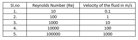
Reynolds number = `(rho*V*D)/mu`

Velocity (V) = `(Re*mu)/(rho*D)`

Calculated Velocity for the given Reynolds number is as follows.

Geometry Setup:

• The Ansys Workbench software was launched and under the Analysis systems "Fluid Flow (Fluent) was chosen. Rename the project according to the case.
• Right click on the "Geometry" and select "Edit Geometry in SpaceClaim" and Create the geometry as per the dimensions.

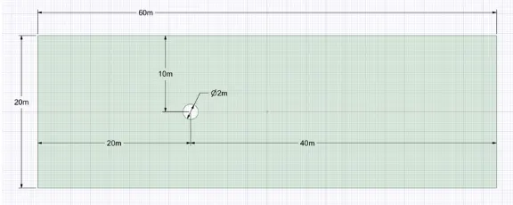
• 2D geometry for flow over a cylinder is prepared in spaceclaim, with 2 m cylinder diameter, 20 m upstream distance, 40 m of downstream distance and 10 m distance above and below the cylinder. All distances are from the centre of cylinder.

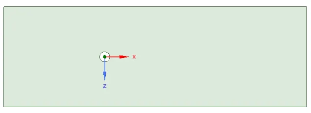
• Once the geometry preparation is done, we have to create a named selection and meshing parameters under the Mesh category.
• For creating the named selection Edge selection is enabled and the selected edges are named.
• In order to create a fine mesh and to obtain the flow properties around the cylinder certain meshing properties are used.
• Added to that an inflation parameter is used around the cylinder in order to get the flow properties accurately.

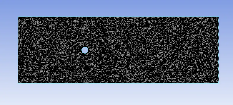
• The element size is to set to 0.25 m and a total of 6 inflation layers have been set.

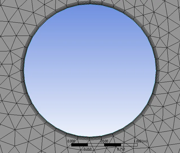
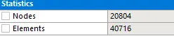
Mesh Statistics:

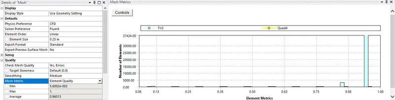
Mesh Quality and Mesh Metrics:

After setting up the mesh close the mesh tab and update the mesh category for further proceedings.

Case Setup:

• In setup the simulation settings are done. For this simulation we are using Laminar model for simulating the flow as we are targeted to use less values Reynolds number.
• For the Part 1-a we will be using Steady state solver and for the Part 1-b we will be using Transient state solver and for the remaining simulation Steady state solver is used.
• A user defined material was created in order to simulate the flow.
• Material used in cellzone is changed to user defined material.
• Inlet Boundary conditions are assigned as per the case.
• Reference parameters are updated as per inlet BC.
• Monitor point, contours and animation settings are done as per requirement. Under Solution > Reports > Definitions, reports for monitor point velocity, for coefficient of drag and lift are set.
• Solution is initialised with Hybrid settings and thereafter run for required number of iterations.
• The required Post processing is done.
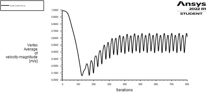
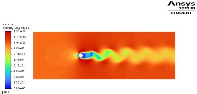
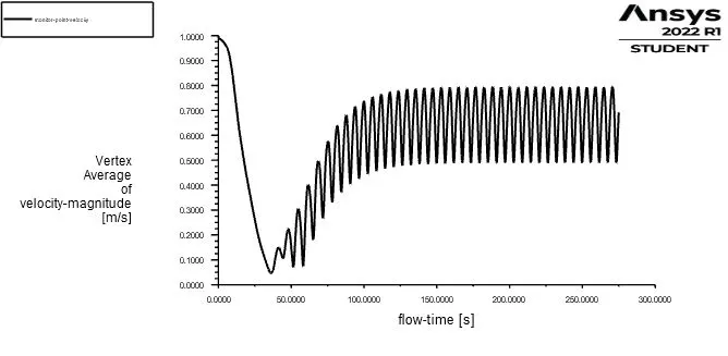
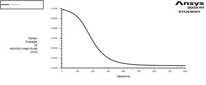
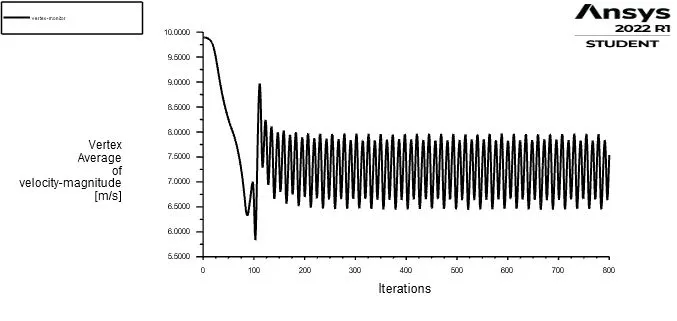
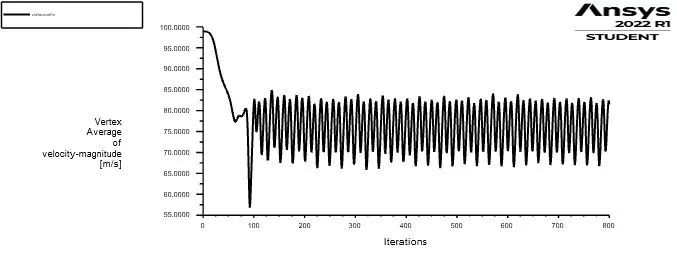
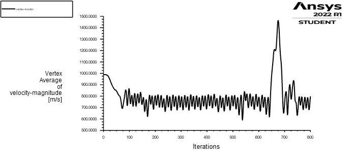
• The monitor point velocity plots show the vortex shedding behind the cylinder.
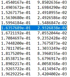
• For Transient simulation FFT for coefficient of Lift is performed to find out Strouhal Number (St).

Part 1-a:

Steady state simulation:

Steady State Simulation for Re = 100

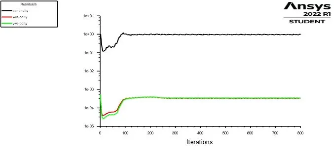
No of iterations = 800

Velocity = 1 m/s

Results:

Residual plot:

Monitor point velocity plot:

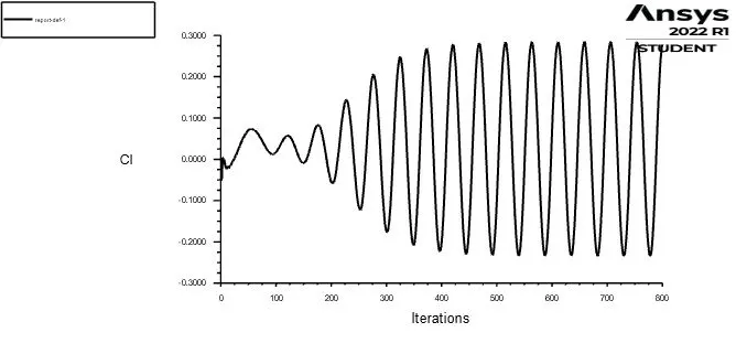
Co-efficient of Lift plot:

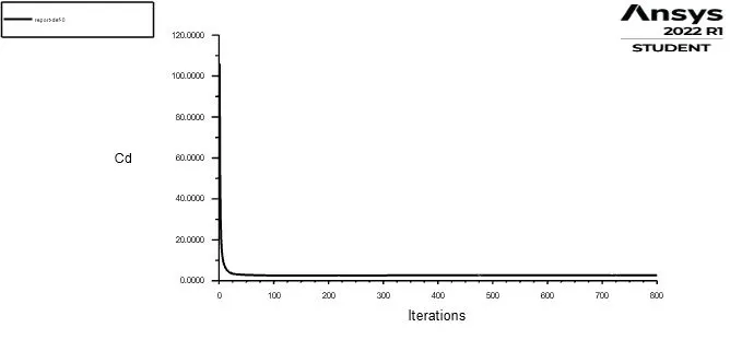
Co-efficient of Drag plot:

Velocity Contour:

Pressure Contour:

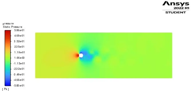
The value for Co-efficient of Drag `C_D = 1.3410828`

The value for Co-efficient of lift `C_L = 0.1390296`

Case 1-b:

Transient State Simulation for Re=100

Time step size = 0.1

Number of Time Steps = 2750

Velocity = 1 m/s

Results:

Residual plot:

Monitor point velocity plot:

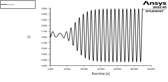
Co-efficient of Lift plot:

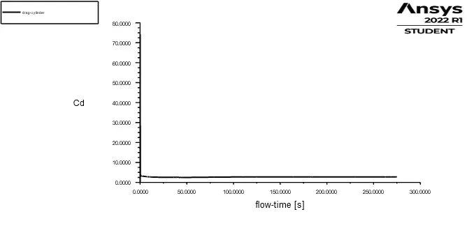
Co-efficient of Drag plot:

Magnitude Vs Strouhal Number plot:

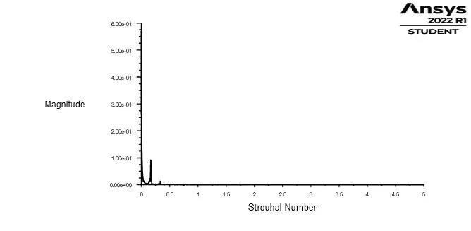
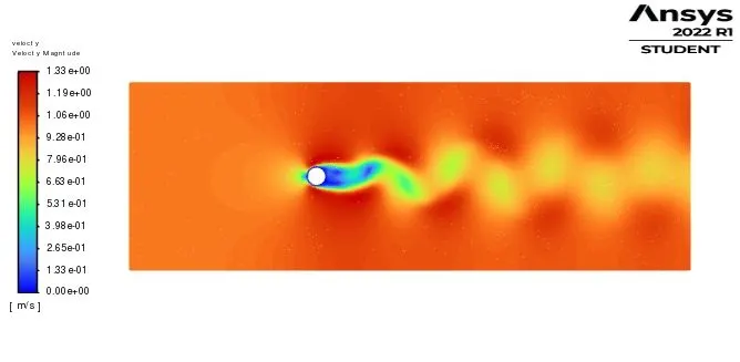
The Value of Strouhal Number from the data written from FFT, is found to be 0.163

Velocity Contour:

Pressure Contour:

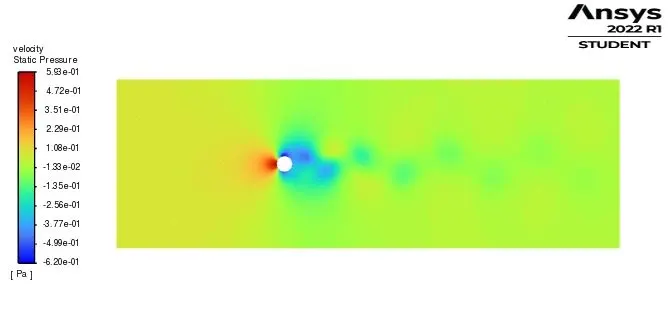
The value for Co-efficient of Drag `C_D = 1.3777103`

The value for Co-efficient of lift `C_L = 0.23341096`

Calculation of coefficient of drag and lift over a cylinder for the Reynolds number to 10,100,1000,10000 &

100000:

Part 2-a:

Steady state simulation:

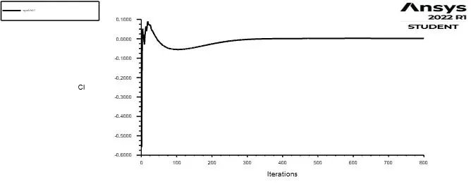
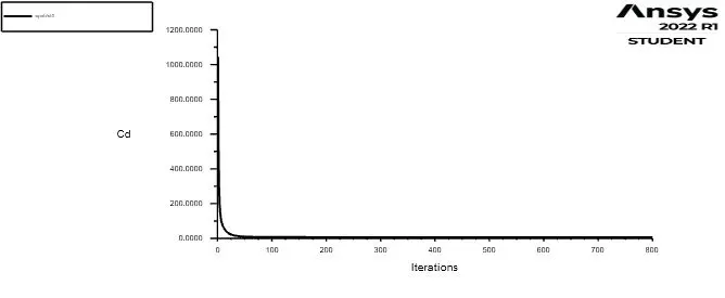
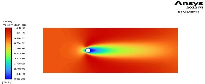
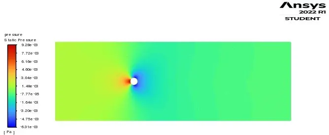
Steady State Simulation for Re = 10

No of iterations = 800

Velocity = 0.1 m/s

Results:

Residual plot:

Monitor point velocity plot:

Co-efficient of Lift plot:

Co-efficient of Drag plot:

Velocity Contour:

Pressure Contour:

Part 2-b:

Steady state simulation:

Steady State Simulation for Re = 100

No of iterations = 800

Velocity = 1 m/s

Results:

Residual plot:

Monitor point velocity plot:

Co-efficient of Lift plot:

Co-efficient of Drag plot:

Velocity Contour:

Pressure Contour:

Part 2-c:

Steady state simulation:

Steady State Simulation for Re = 1000

No of iterations = 800

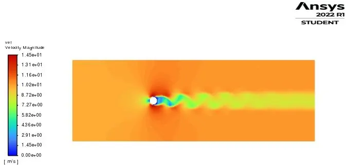
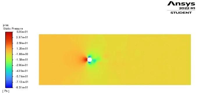
Velocity = 10 m/s

Results:

Residual plot:

Monitor point velocity plot:

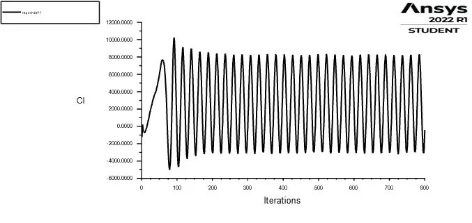
Co-efficient of Lift plot:

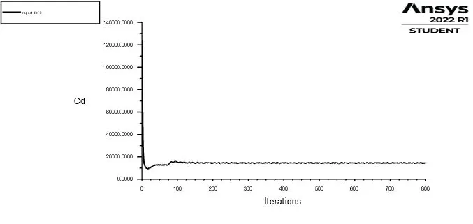
Co-efficient of Drag plot:

Velocity Contour:

Pressure Contour:

Part 2-d:

Steady state simulation:

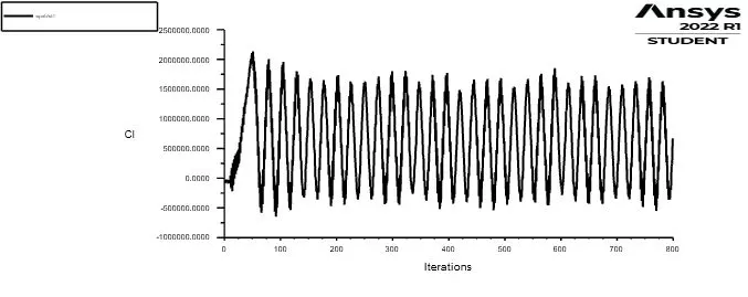
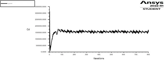
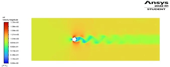
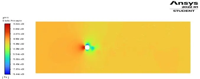
Steady State Simulation for Re = 10000

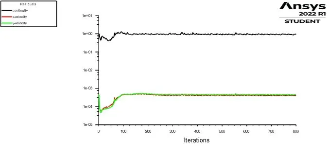
No of iterations = 800

Velocity = 100 m/s

Results:

Residual plot:

Monitor point velocity plot:

Co-efficient of Lift plot:

Co-efficient of Drag plot:

Velocity Contour:

Pressure Contour:

Part 2-e:

Steady state simulation:

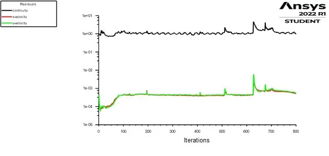
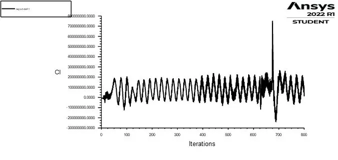
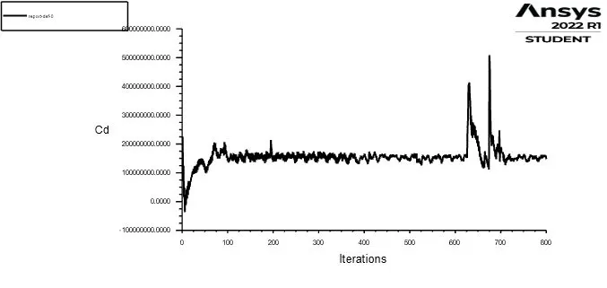
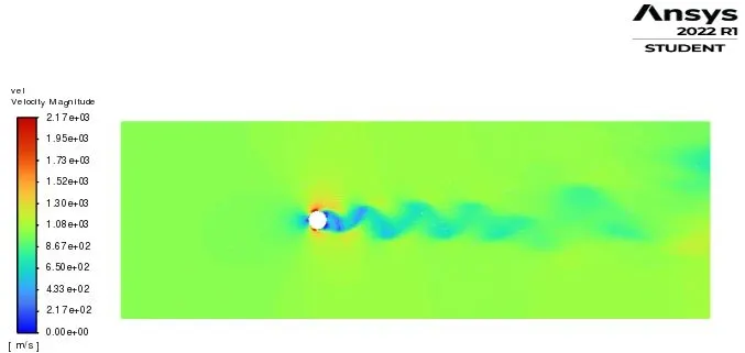
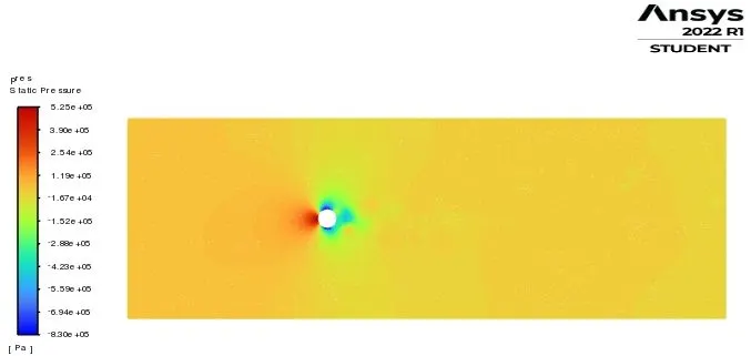
Steady State Simulation for Re = 100000

No of iterations = 800

Velocity = 1000 m/s

Results:

Residual plot:

Monitor point velocity plot:

Co-efficient of Lift plot:

Co-efficient of Drag plot:

Velocity Contour:

Pressure Contour:

Result:

Values of co-efficient of drag and lift co-efficient for respective Reynolds number is tabulated as follows.

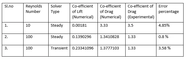
The drag coefficient decreases at low Reynolds numbers because the flow is in a regime called creeping flow. That is, the inertial forces are negligible. Drag is a sum of friction drag and pressure drag. At very low Reynolds number the flow is fully attached, the drag is due to skin friction drag and as Reynolds number increases there will be increase in pressure drag due to separation. When flow turns to turbulent again there the flow will be more attached this causes decrease in pressure drag but eventually leads to increase in friction drag.

Conclusion:

• The flow over a circular cylinder was simulated with different Reynolds number values.
• In the first part under laminar flow conditions both the steady state and transient state simulation was carried out at a Reynold's number of 100. The Strouhal number is calculated for unsteady case.
• Drag and lift coefficients are calculated for both the cases. In that particular Reynold's number, Von Karman Vortex Shedding is visualized and understood.
• In the second part at different Reynold's number, steady state simulations are set-up to visualize vortex shedding and the effect on drag and lift coefficients.
• For Re=10, it is observed that there is no formation of vortex shedding and in the rest of the cases, it is clearly observed.
• There is significant effect of Reynolds number over drag coefficient. The drag coefficient is significantly reduced past a increment in Reynolds number.
• At higher Reynolds number skin-friction drag contributes more to total drag and leads to heating of the surface, however at lesser Reynolds number pressure drag accounts for more in total drag.
• Contours plots of velocity and pressure are displayed for different values of Reynolds number.