Week 2 - Flow over a Cylinder.

OBJECTIVE

To simulate the flow over a cylinder and explain the phenomenon of Karman vortex street.

PART-I

1. Simulate the flow with the steady and unsteady case and calculate the Strouhal Number for Re= 100.

PART-II

Calculate the coefficient of drag and lift over a cylinder by setting the Reynolds number to 10,100,1000,10000 & 100000. (Run with steady solver) and to discuss the effect of Reynolds number on the coefficient of drag

THEORY

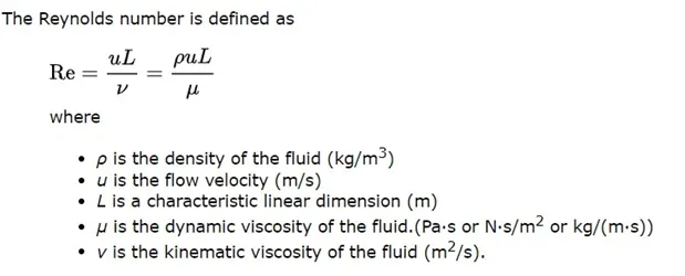
• Reynold's Number

The Reynolds number (Re) is a dimensionless number which helps predict flow patterns in different fluid flow situations. At low Reynolds numbers ( upto 2300), flows tend to be dominated by laminar (sheet-like) flow, while at high Reynolds numbers (greater than 4000) flows tend to be turbulent. For 2300<Re<4000, the flow is in transition zone.

• Strouhal Number

The Strouhal number is a dimensionless number describing oscillating flow mechanisms.

The Strouhal number is often given as

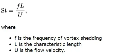
For large Strouhal numbers (order of 1), viscosity dominates fluid flow, resulting in a collective oscillating movement of the fluid "plug". For low Strouhal numbers (order of 10⁻⁴ and below), the high-speed, quasi-steady-state portion of the movement dominates the oscillation. Oscillation at intermediate Strouhal numbers is characterized by the buildup and rapidly subsequent shedding of vortices

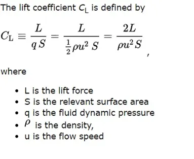
• Coefficient of Lift

The lift coefficient (C_L) is a dimensionless quantity that relates the lift generated by a lifting body to the fluid density around the body, the fluid velocity and an associated reference area. C_L is a function of the angle of the body to the flow, its Reynold's number and its Mach number.

• Coefficient of Drag

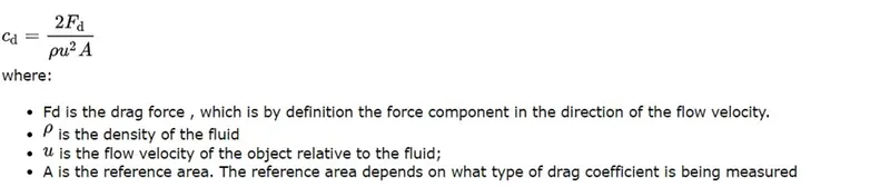
The drag coefficient (Cd) is a dimensionless quantity that is used to quantify the drag or resistance of an object in a fluid environment, such as air or water. A lower drag coefficient indicates the object will have less aerodynamic or hydrodynamic drag. The drag coefficient is always associated with a particular surface area.

The drag coefficient Cd is defined as

PROCEDURE/WORKFLOW

• GEOMETRY

Since we are simulating a 2D flow, a circle of 2m diameter is drawn within a rectangular domain of 60*20m. Make sure that the units are changed to meters in Spaceclaim.

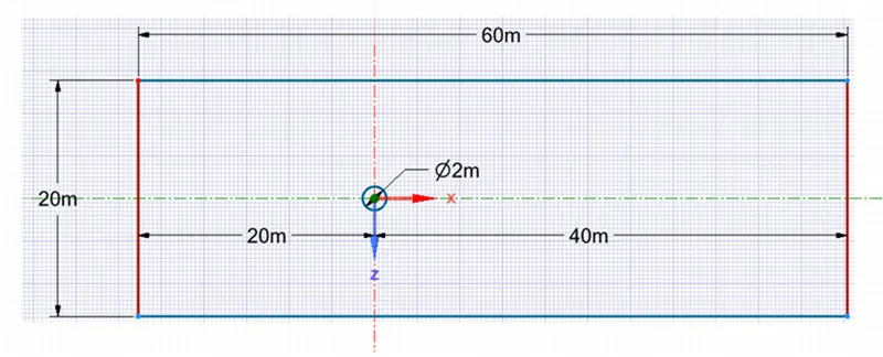
Figure 1: Geometric setup of 2D cylinder simulation with rectangular domain

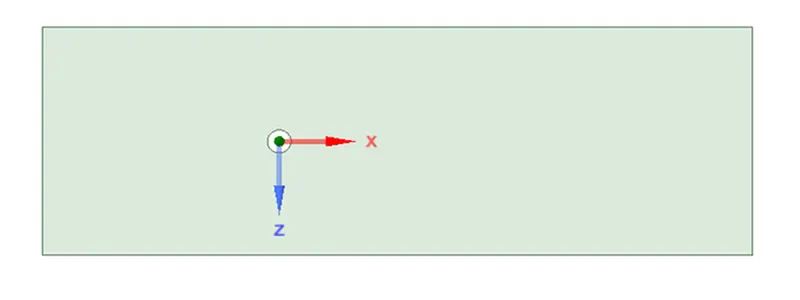
Figure 2: Final geometric setup of 2D cylinder simulation with rectangular domain for simulation

• MESHING
• Create named selections as per convenience.
• Generate mesh.
• Insert method->select geometry->triangular
• Change element size accordingly (final element size=0.25m)
• Insert sizing->select edges->no: of divisions =36.
• Insert inflation->select the body as geometry and circular surface as boundary->first layer thickness->provide thickness accordingly (5e-3)->inflation layers =10.

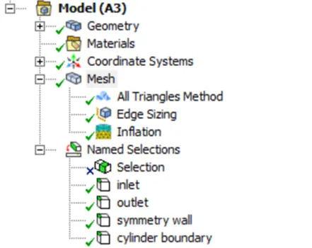
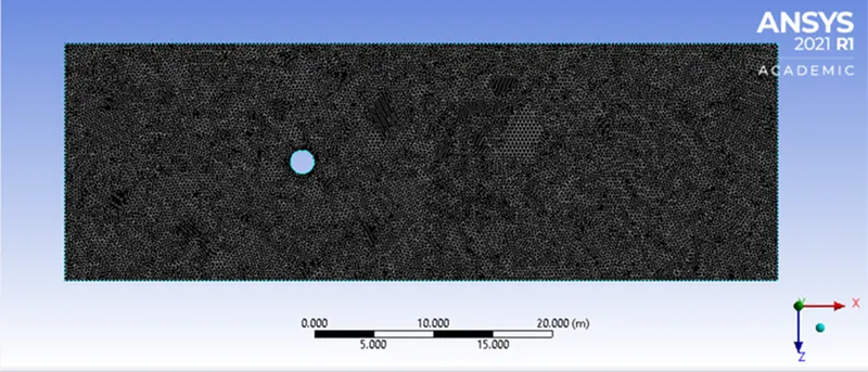
Figure 3: Meshed domain

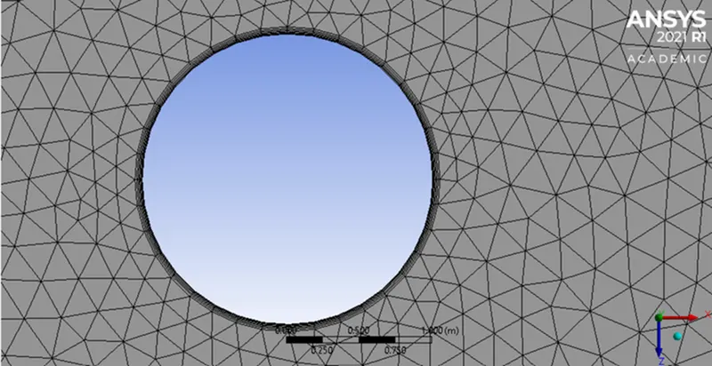
Figure 4:

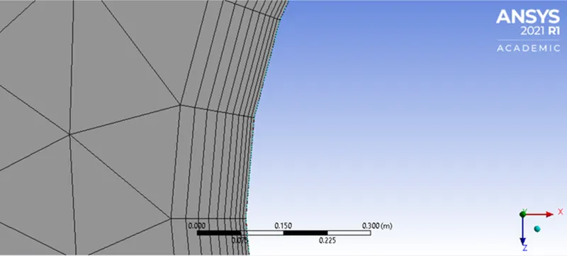
Figure 4 & 5: Meshed domain with inflation layers.

• SETUP
• Make sure that double precision and parallel processors are checked.
• Perform mesh check.
• General->pressure-based, velocity solvers are selected.
• Since we conduct steady state simulation, check steady in time. Later transient is checked for unsteady simulation

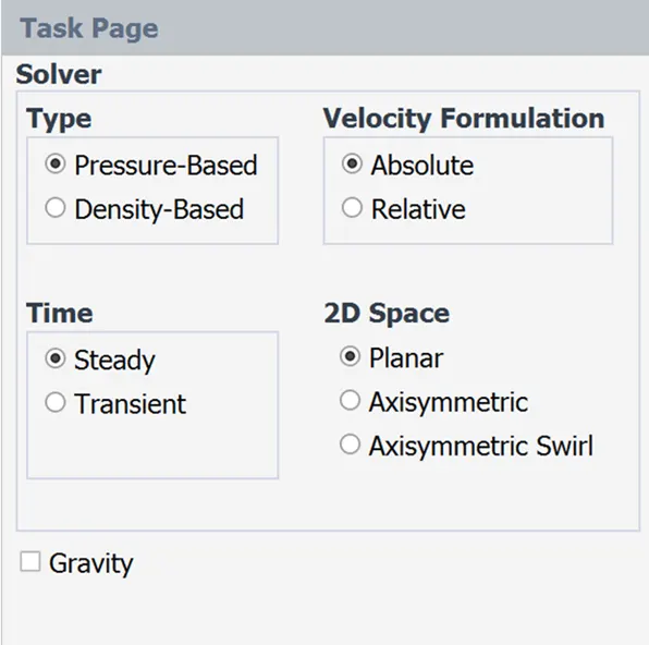
• Physics->viscous->laminar
• 

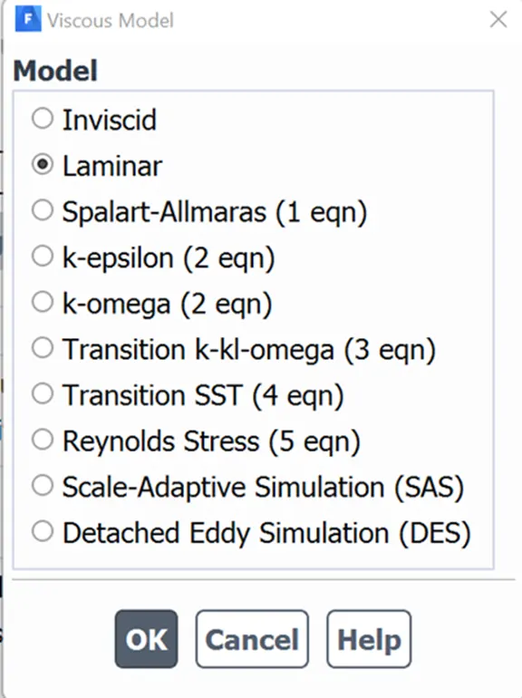
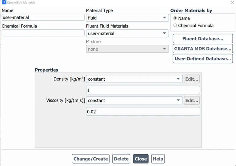
• Materials->fluent data base->select air->copy and rename->ok-> delete the rest of the components in the dropdown after changing the material in cell zones as the one renamed.
• Change the density value as 1Kg/m^3 and dynamic viscosity as 0.02 Kg/m-s and click create/change.

• Boundary conditions
• Inlet velocity 1m/s (later changed to get different Reynolds numbers)
• Cylinder wall-no slip
• Symmetry wall-type symmetry
• Outlet - no change
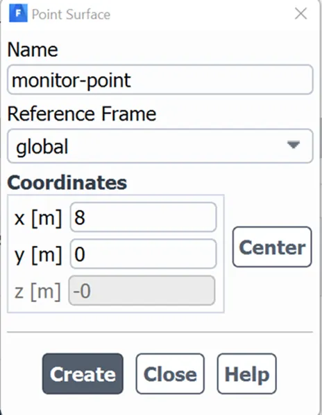
• Creating monitor point
• Results(post-processing)->create->point->rename->provide the location as 8->create

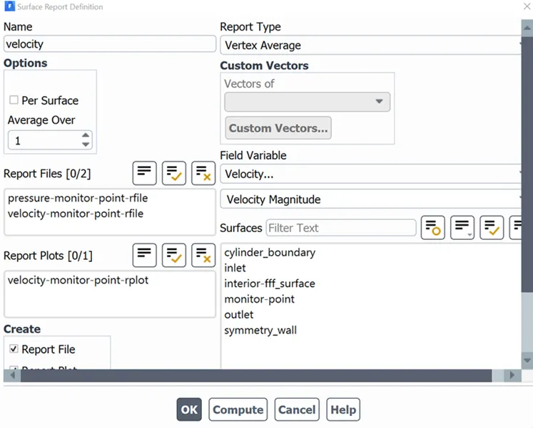
• Creating surface reports
• Solutions->->definitions->new->surface report->vertex average->rename-> select velocity->select monitor-point
• Similarly create the pressure plot at monitor point

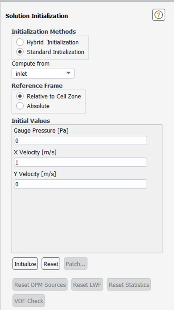
• INITIALIZATION
• Standard initialization-> compute from inlet->initialize
• 

• Creating Contour plots
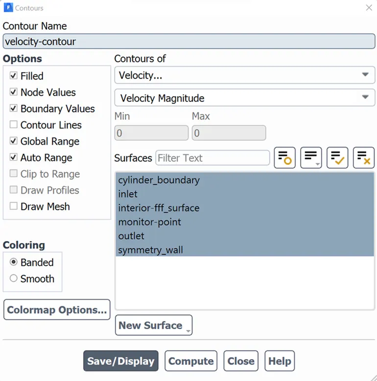
• Results->contours->new->new->rename->select velocity->filled->select everything->save and display->compute
• Similarly create the pressure contour
• 

• Creating animation
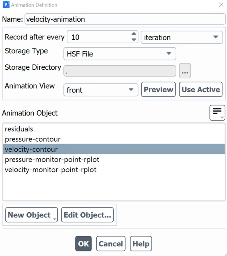
• Solution->activities->create->->solution animation->rename->update after 10 iterations->select velocity contour->ok
• 

• RUN CALCULATION
• For steady flow, run the simulation with 350 iterations.
• For transient flow simulation, run with a time step of 0.1 and 500 iterations.

RESULTS AND PLOTS

• Part 1

• Steady state flow with Re =100

Parameter	Value
v	1 m/s
ρ	1 Kg/m^3
μ	0.02 Kg/(m·s)
d	2 m

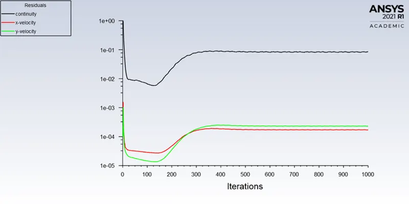
Figure 6: Residual plot for steady flow at Re=100

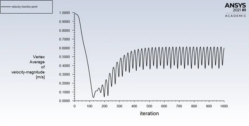
Figure 7: Magnitude of velocity at monitor point for steady flow at Re=100

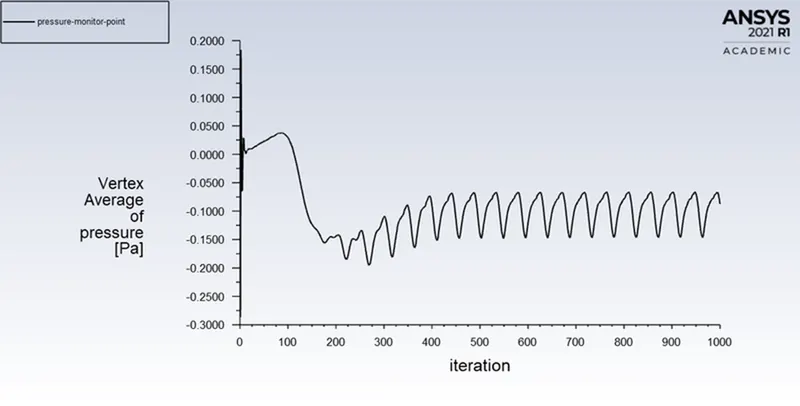
Figure 8: Magnitude of pressure at monitor point for steady flow at Re=100

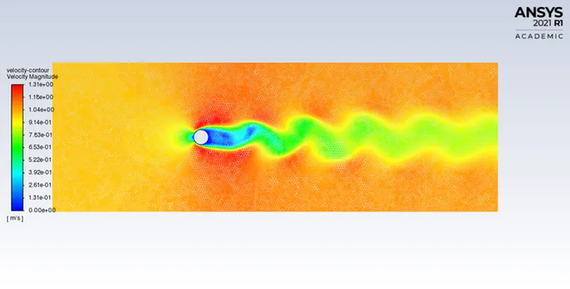
Figure 9: Velocity contour for steady flow at Re=100

• Transient state flow with Re =100

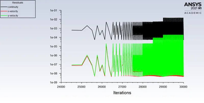
Figure 10: Residual plot for transient flow at Re=100

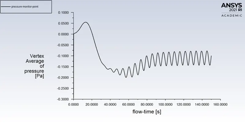
Figure 11: Magnitude of pressure at monitor point for transient flow at Re=100

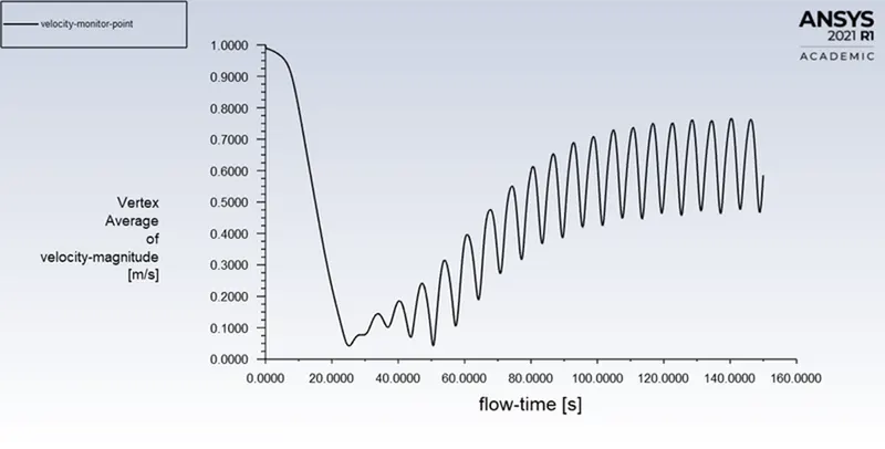
Figure 12: Magnitude of velocity at monitor point for transient flow at Re=100

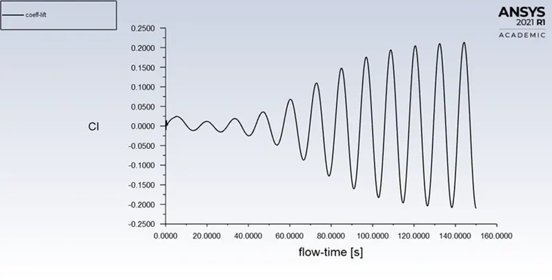
Figure 13: Coefficient of lift for transient flow at Re=100

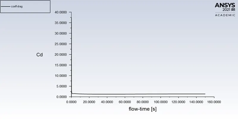
Figure 14: Coefficient of drag for transient flow at Re=100

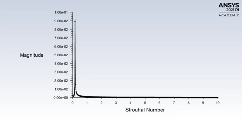
Figure 15: Strouhal number for transient flow at Re=100

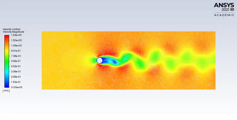
Figure 16: Velocity contour for transient flow at Re=100

• Part 2
• Steady flow
• Re=10

Parameter	Value
v	0.1 m/s
ρ	1 Kg/m^3
μ	0.02 Kg/(m·s)
d	2 m

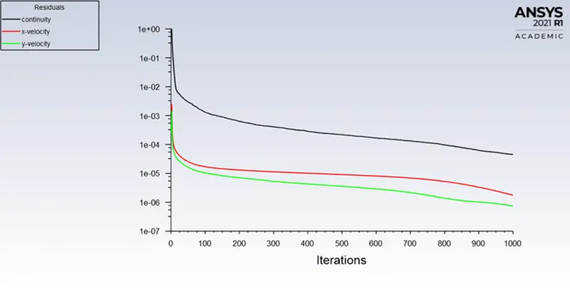
Figure 17: Residual plot for steady flow at Re=10

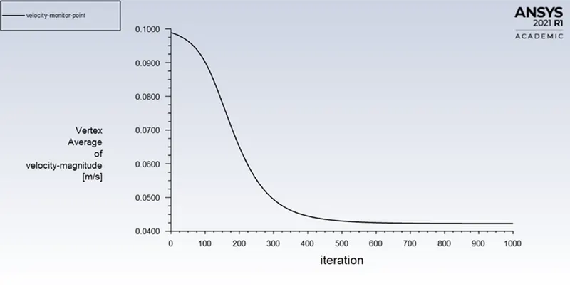
Figure 18: Magnitude of velocity at monitor point for steady flow at Re=10

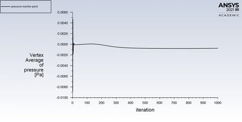
Figure 19: Magnitude of pressure at monitor point for steady flow at Re=10

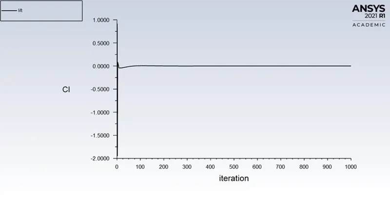
Figure 20: Coefficient of lift for steady flow at Re=10

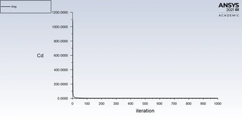
Figure 21: Coefficient of drag for steady flow at Re=10

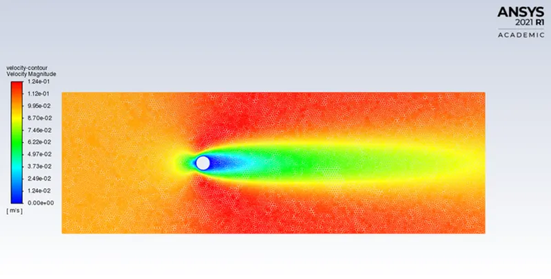
Figure 22: Velocity contour for steady flow at Re=10

• Re=100

Parameter	Value
v	1 m/s
ρ	1 Kg/m^3
μ	0.02 Kg/(m·s)
d	2 m

Figure 23: Residual plot for steady flow at Re=100

Figure 24: Magnitude of velocity at monitor point for steady flow at Re=100

Figure 25: Magnitude of pressure at monitor point for steady flow at Re=100

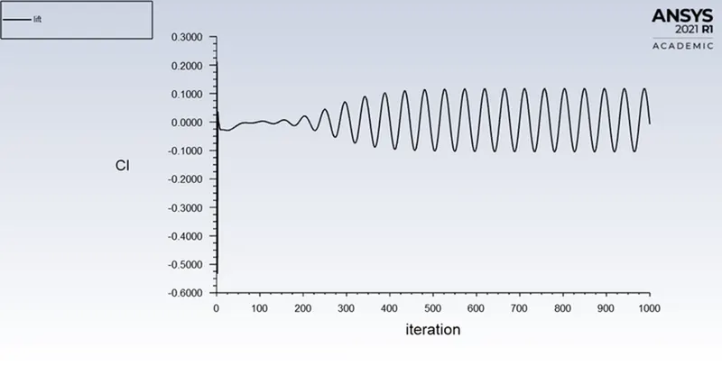
Figure 26: Coefficient of lift for steady flow at Re=100

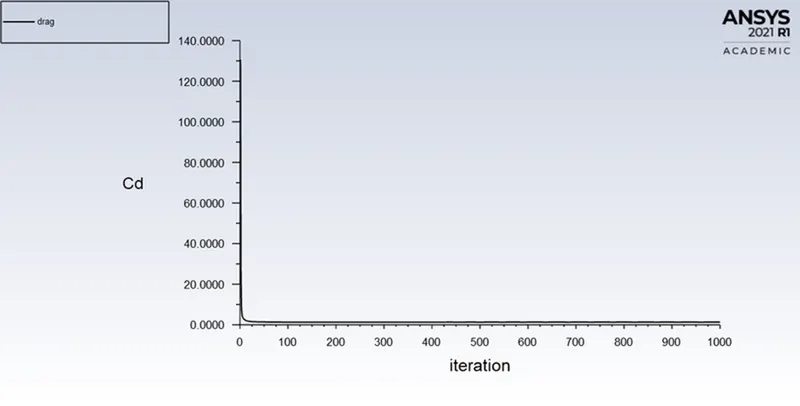
Figure 27: Coefficient of drag for steady flow at Re=100

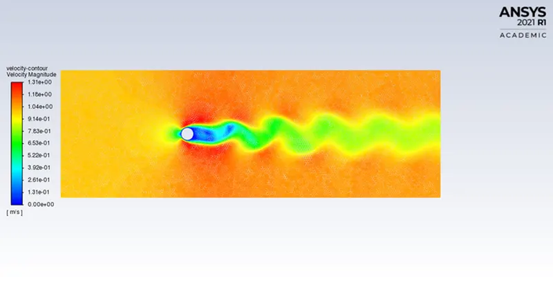
Figure 28: Velocity contour for steady flow at Re=100

• Re=1000

Parameter	Value
v	10 m/s
ρ	1 Kg/m^3
μ	0.02 Kg/(m·s)
d	2 m

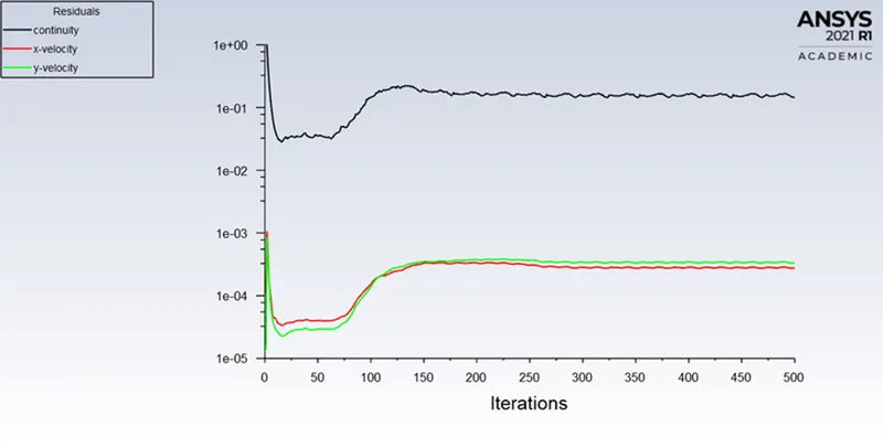
Figure 29: Residual plot for steady flow at Re=1000

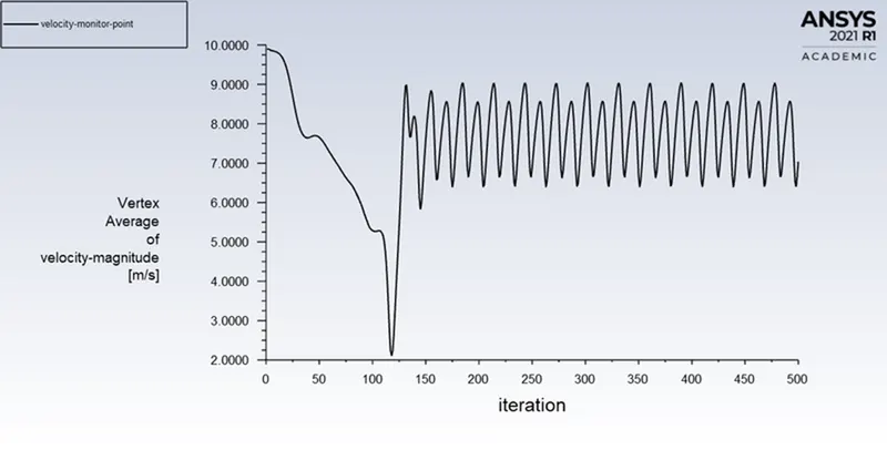
Figure 30: Magnitude of velocity at monitor point for steady flow at Re=1000

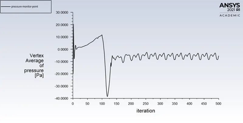
Figure 31: Magnitude of pressure at monitor point for steady flow at Re=1000

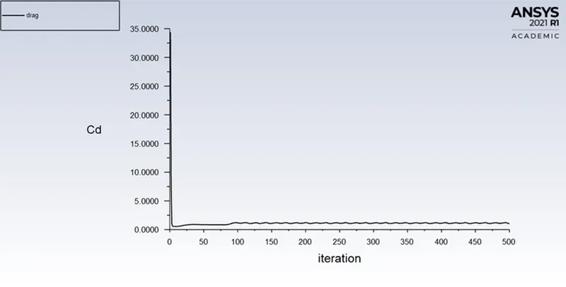
Figure 32: Coefficient of drag for steady flow at Re=1000

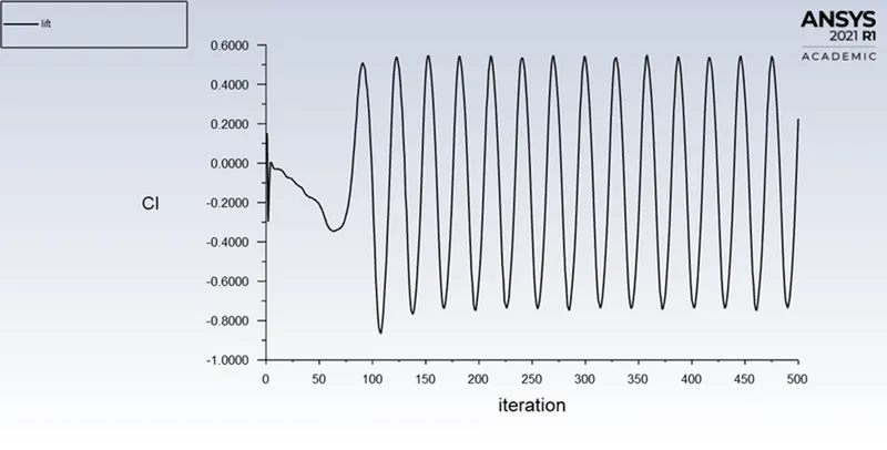
Figure 33: Coefficient of lift for steady flow at Re=1000

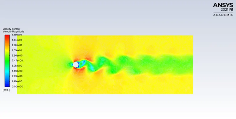
Figure 34: Velocity contour for steady flow at Re=1000

• Re=10000

Parameter	Value
v	100 m/s
ρ	1 Kg/m^3
μ	0.02 Kg/(m·s)
d	2 m

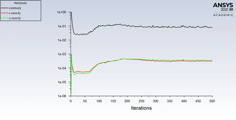
Figure 35: Residual plot for steady flow at Re=10000

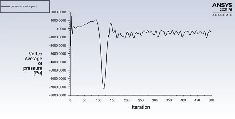
Figure 36: Magnitude of pressure at monitor point for steady flow at Re=10000

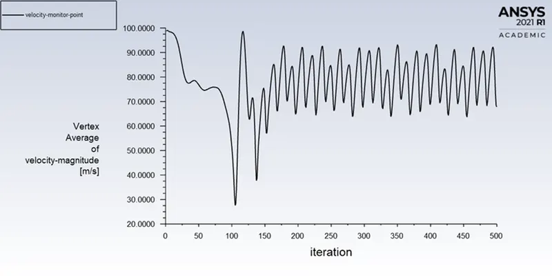
Figure 37: Magnitude of velocity at monitor point for steady flow at Re=10000

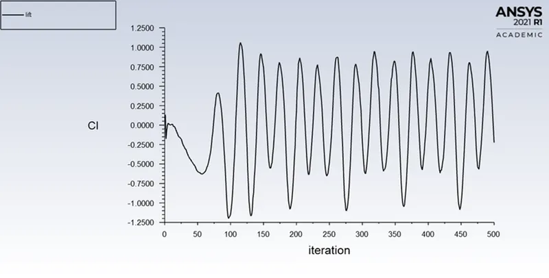
Figure 38: Coefficient of lift for steady flow at Re=10000

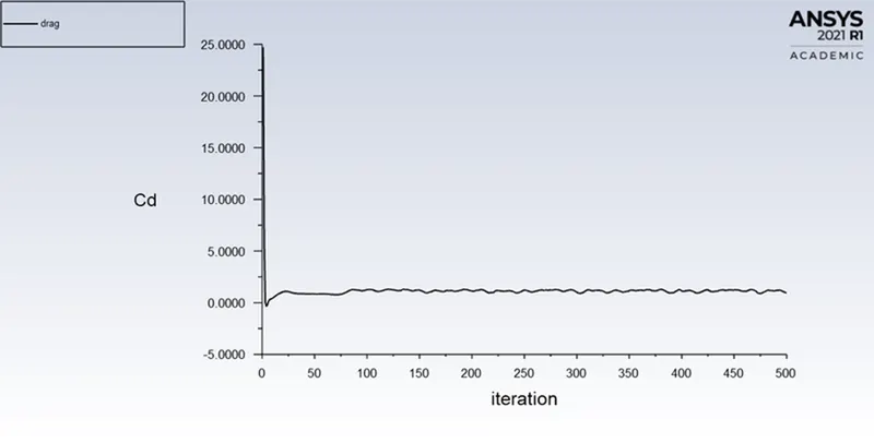
Figure 39: Coefficient of drag for steady flow at Re=10000

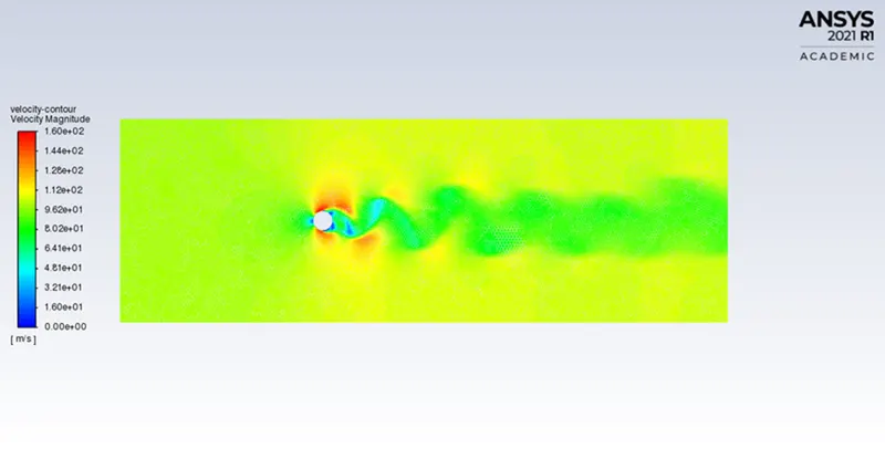
Figure 40: Velocity contour for steady flow at Re=10000

• Re=1,00,000

Parameter	Value
v	1000 m/s
ρ	1 Kg/m^3
μ	0.02 Kg/(m·s)
d	2 m

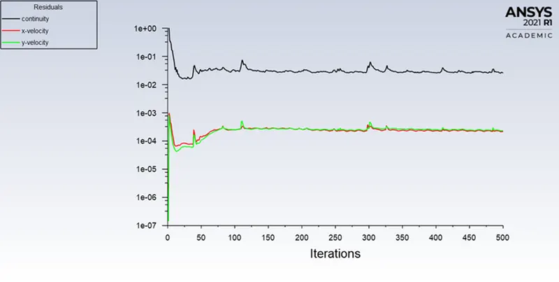
Figure 41: Residual plot for steady flow at Re=100000

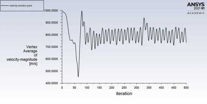
Figure 42: Magnitude of velocity at monitor point for steady flow at Re=100000

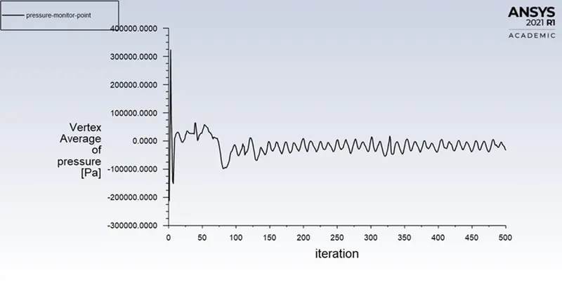
Figure 43: Magnitude of pressure at monitor point for steady flow at Re=100000

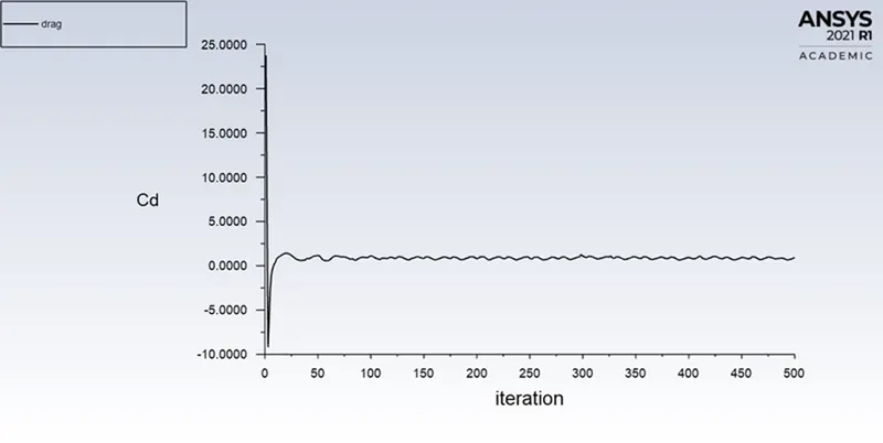
Figure 44: Coefficient of drag for steady flow at Re=100000

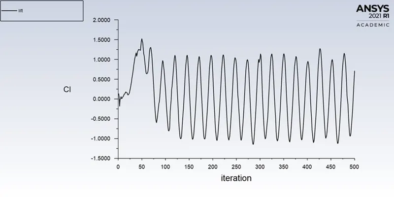
Figure 45: Coefficient of lift for steady flow at Re=100000

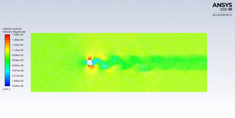
Figure 46: Velocity contour for steady flow at Re=100000

Re	Cd
10	3.325471
100	1.308483
1000	1.139917
10,000	1.139209
1,00,000	0.8025

Table 1: Coefficient of drag values for varying Reynold's numbers

• The 2D Coefficient of drag at Re = 100 is 1.3353[1].

The percentage error for Cd is [ (1.3353-1.308483)/1.3353 ]*100=2.0083%

• The Strouhal number for transient simulation at Re=100 is 9.2e-3

CONCLUSIONS

• As the Reynolds number is increasing, it can be seen that the vortices are shed at a particular frequency from upper and lower surface of the cylinder, which is actually a property of Reynolds number.
• As the Reynolds number increases, (greater than 1000), inertial forces dominate the viscous force and the oscillations start to increase.
• Also, the coefficieny of drag shows a decreasing trend with increasing Reynolds number.
• The transient state simulation is more suitable to analyse flow over a cylinder as it is time-dependent and more accurate.
• The obtained Strouhal number falls in the intermediary range which is characterised by the buildup and rapidly subsequent shedding of vortices, which is clearly visible from the plots

REFERENCE

[1]B.N. Rajani, A. Kandasamy, Sekhar Majumdar, ' Numerical Simulation of laminar flow past a circular cylinder', Applied Mathematical Modelling (2009), pages 1228-1247, https://doi.org/10.1016/j.apm.2008.01.017