Steady vs Unsteady flow over a Cylinder using Ansys Fluent.

Aim: Steady vs Unsteady flow over a Cylinder.

Theory:

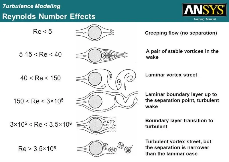
Flow over a cylinder is a classical problem for understanding the flow over an obstacle. The geometry of the cylinder is simple and allows us to understand all the complexities that occur and turbulence for different Reynolds Numbers. Reynolds Number helps us to understand the flow patterns of the different fluid flow situations. The different range of Reynolds Numbers represents different flow patterns. At low Reynolds Numbers, the flow pattern is observed to be Laminar i.e., Smooth, Constant fluid motion. At higher Reynolds Numbers the flow pattern is observed to be Turbulent i.e., Chaotic eddies, Vortices, and Flow instabilities. In this project, we will try to understand the variation of velocity and pressure in certain flow directions for different Reynolds Numbers by simulating it with proper boundary conditions, Mesh sizing, and Convergence criteria using Ansys Fluent Flow Simulation.

Objective: Simulate the flow over a cylinder and explain the phenomenon of Karman Vortex Street.

PART-I
1. Simulate the flow with the steady and unsteady case and calculate the Strouhal Number for Re=100.

PART-II
1. Calculate the coefficient of drag and lift over a cylinder by setting the Reynolds number to 10,100,1000,10000 & 100000. (Run with steady solver)

2. Discuss the effect of Reynolds number on the coefficient of drag. Results should be validated with any standard literature and error should be within 5%]


Expected results:

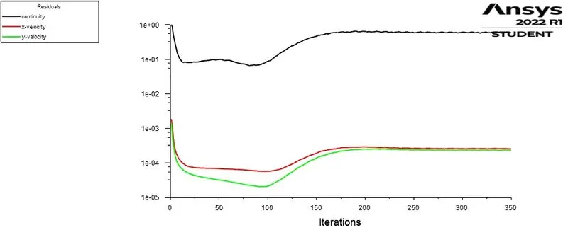
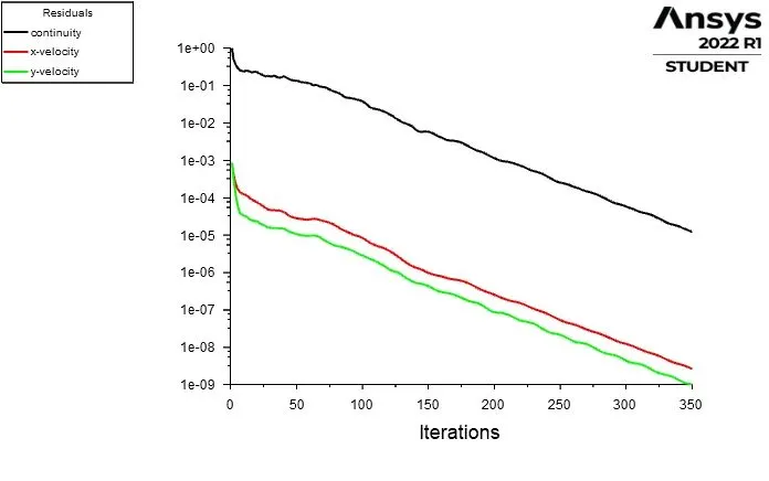
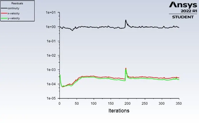
1. In both approaches, show that the flow has converged. That is, what quantities or plots need to be looked at to determine that the flow has converged?
2. Plots of the coefficient of drag and lift.
3. Plots to show vortex shedding behind the cylinder.
4. Mention the preferred material at the end of the challenge submission page.

Vortex shedding:

It is an oscillating flow that takes place when a fluid such as air or water flows past a bluff (as opposed to streamlined) body at certain velocities, depending on the size and shape of the body. In this flow, Vortices are created at the back of the body and detach periodically from either side of the body, forming a von Karman vortex street. The fluid flow past the object creates alternating low-pressure vortices on the downstream side of the object. The object will tend to move toward the low-pressure zone. Moreover, von Kármán vortex street is a repeating pattern of swirling vortices, caused by a process known as vortex shedding, which is responsible for the unsteady separation of flow of a fluid around blund bodies.

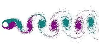
In fluid dynamics, a Kármán vortex street (or a von Kármán vortex street) is a repeating pattern of swirling vortices, caused by a process known as vortex shedding, which is responsible for the unsteady separation of flow of a fluid around blunt bodies.

A vortex street will form only at a certain range of flow velocities, specified by a range of Reynolds number (Re), typically above a limiting Re value of about 90. The (global) Reynolds number for a flow is a measure of the ratio of inertial to viscous forces in the flow of a fluid around a body or in a channel, and may be defined as a nondimensional parameter of the global speed of the whole fluid flow:

Strouhal number: It is a dimensionless number describing oscillating flow mechanisms.

The Strouhal number is an integral part of the fundamentals of fluid mechanics.

The Strouhal number is often given as

where f is the frequency of vortex shedding,

L is the characteristic length,

U is the flow velocity.

Drag coefficient:

In fluid dynamics, drag is a force acting opposite to the relative motion of any object moving with respect to a surrounding fluid. This can exist between two fluid layers or between a fluid and a solid surface. Unlike other resistive forces, such as dry friction, which are nearly independent of velocity, the drag force depends on velocity.

In fluid dynamics, the drag coefficient is a dimensionless quantity that is used to quantify the drag or resistance of an object in a fluid environment,

The drag coefficient is defined as:

where:

• is the drag force, which is by definition the force component in the direction of the flow velocity;
• is the mass density of the fluid;
• is the flow speed of the object relative to the fluid;
• is the reference area.

Lift coefficient:

The lift coefficient (C_L) is a dimensionless quantity that relates the lift generated by a lifting body to the fluid density around the body, the fluid velocity and an associated reference area.

The lift coefficient C_L is defined by

,

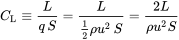where is the lift force,

is the relevant surface area,

is the fluid dynamic pressure, in turn linked to the fluid density , and to the flow speed .

Reynolds number (Re):

It helps predict flow patterns in different fluid flow situations. At low Reynolds numbers, flows tend to be dominated by laminar flow, while at high Reynolds numbers flows tend to be turbulent. The turbulence results from differences in the fluid's speed and direction, which may sometimes intersect or even move counter to the overall direction of the flow (eddy currents). These eddy currents begin to churn the flow, using up energy in the process, which for liquids increases the chances of cavitation. Reynolds numbers are an important dimensinonless quantity in fluid mechanics. The Reynolds number has wide applications, ranging from liquid flow in a pipe to the passage of air over an aircraft wing. It is used to predict the transition from laminar or turbulent flow, and is used in the scaling of similar but different-sized flow situations, such as between an aircraft model in a wind tunnel and the full size version. The predictions of the onset of turbulence and the ability to calculate scaling effects can be used to help predict fluid behaviour on a larger scale, such as in local or global air or water movement and thereby the associated meteorological and climatological effects.

With respect to laminar and turbulent flow regimes:

• laminar flow occurs at low Reynolds numbers, where viscous forces are dominant, and is characterized by smooth, constant fluid motion;
• turbulent flow occurs at high Reynolds numbers and is dominated by inertial forces, which tend to produce chaotic eddies, vortices and other flow instabilities.

The Reynolds number is defined as:

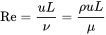
where:

• ρ is the density of the fluid ( kg/m³)
• u is the flow speed (m/s)
• L is a characteristic linear dimension (m)
• μ is the dynamic viscosity of the fluid (Pa·s or N·s/m² or kg/(m·s))
• ν is the kinematic viscosity of the fluid (m²/s).

Understanding the flow over cylinder by considering following illustration:

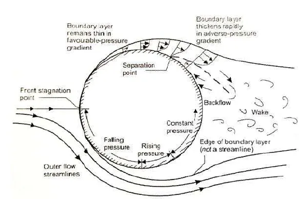
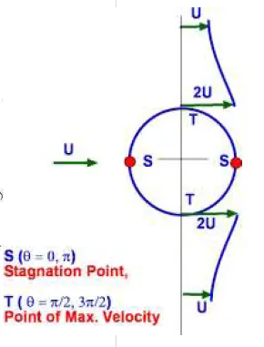
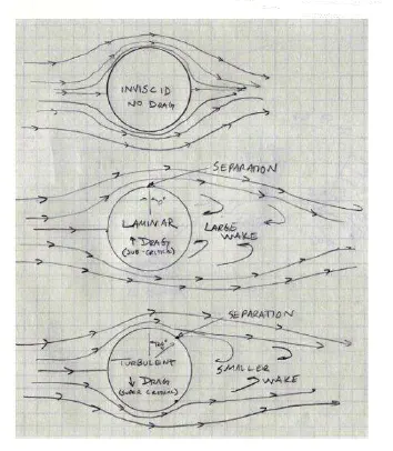
From the above there are some terms that need to be discussed:

1. Signation Point
2. Point of Maximum velocity
3. Boundary-Layer
4. Flow Separation
5. Wake.

Boundary-Layer:

A boundary layer is the layer of fluid in the immediate vicinity of bonding surfare where the effers of viscosity are significant. The viscous nature of airflow reduces the local velocities on surface and is responsible for skin friction. The layer of air over the wing's surface that is slowed down or stopped by viscosity, is the boundary layer. There are two different types of boundary layer flow: laminar and turbulent.

Laminar boundary layer flow:

The laminar boundary is a very smooth flow, while the turbulent boundary layer contains swirls or 'eddies'. The laminar flow creates less skin friction drag than the turbulent flow but is less stable. Boundary layer flow over a wing surface begins as a smooth laminar flow. As the flow continues back from the leading edge, the laminar boundary layer increases in thickness.

Turbulent boundary layer flow:

At some distance back from the leading edge, the smooth laminar flow breaks down and transitions to a turbulent flow. From a drag standpoint, it is advisable to have the transition from laminar to turbulent flow as far aft on the wing as possible or have large amount of the wing surface within the laminar portion of the boundary layer. The low energy laminar flow, however, tends to break down more suddenly than the turbulent layer.

Flow separation:

It is important to understand when and why the flow separates when fluid flows through the obstacle or cylinder in this case. In boundary layer, due to viscosity, there is a change in pressure along the surface of the body. This causes the boundary layer to be sensitive to the pressure gradient [as the form of a pressure force acting upon fluid particles.] If the pressure decreases in the direction of the flow, the pressure gradient said to be favorable. In this case, the pressure force can assist the fluid movement and there's no flow retardation. However, if the pressure is increasing in the direction of the flow. an adverse pressure gradient condition as so it is called exist. In addition to the presence of a wrong viscous force, the fluid particle now have to move against the increasing pressure force. Therefore,the fluid particles could be stopped or reversed, causing the nighboring particles to move away from the surface. This phenomenon is called the boundary layar separation or flow separation.

Wake:

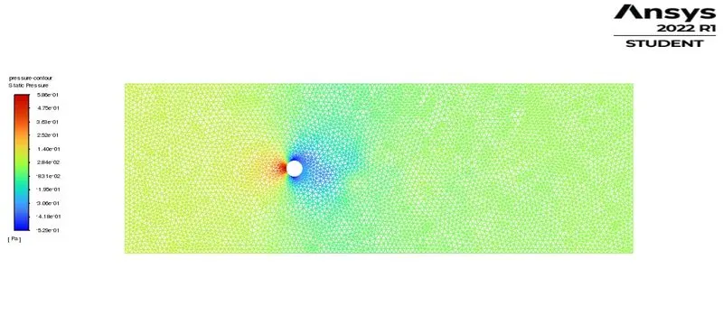
Consider a fluid particle flows within the boundary layer around the circular cylinder. From the pressure distrution measured in an earlier experiment, the pressure is a maximum at the stagnation point and gradually decreases along the front half of the cylinder. The flow stays attached in his favorable pressure region as expected.However, the pressure starts to increase in the rear half of the cylinder and the particle now experiences an adverse pressure gradient. Consequently, the flow separates from the surface and creating a highly turbulent region behind the cylinder called the wake. The pressure inside the wake region remains low as the flow separates and a net pressure force (pressure drag) is produced.

Stagnation Point:

In fluid dynamics, a stagnation point is a point in a flow field where the local velocity of the fluid is zero

Point of Muximum velocity:

Point of maximun velocity is termed where velocity is maximum.

Before proceding with the flow simulation it is important to have an understanding of how different Reynolds Numbers affect the flow:

Procedure:

Geometry:

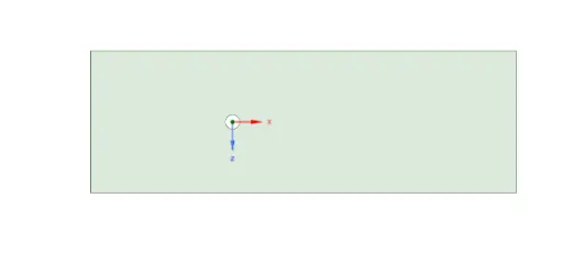
1.Create the geometry by using the line and circle command. Circle diameter of 2 meter and dimension having 20*60m and the circle is placed 20m from the inlet.

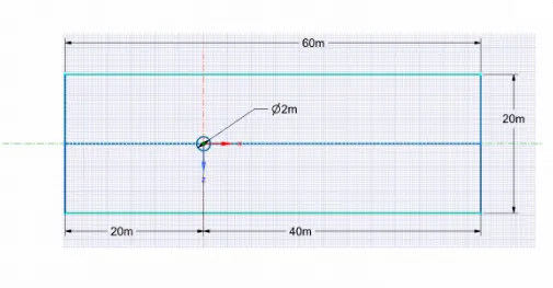
2.Converting the geometry into the surface by using command pull and select. Also, delete the inside the circle to carry out the simulation.

Mesh:

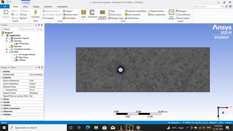
1.First of all, the baseline mesh auto-generate quadrilateral mesh was created. After that, we will change it according to simulation requirements, and it was finely tuned with the help of triangular mesh generated. The model is meshed with an element size of 0.5m.

2.But in the meshing nodes, the shape is more quadrilateral than the triangle so we need to change it by changing the method to the triangle in the insert option.

3.After changing the node's shape into triangles we should improve the mesh around the cylinder by sizing in the mesh which is used to control precisely the mesh.

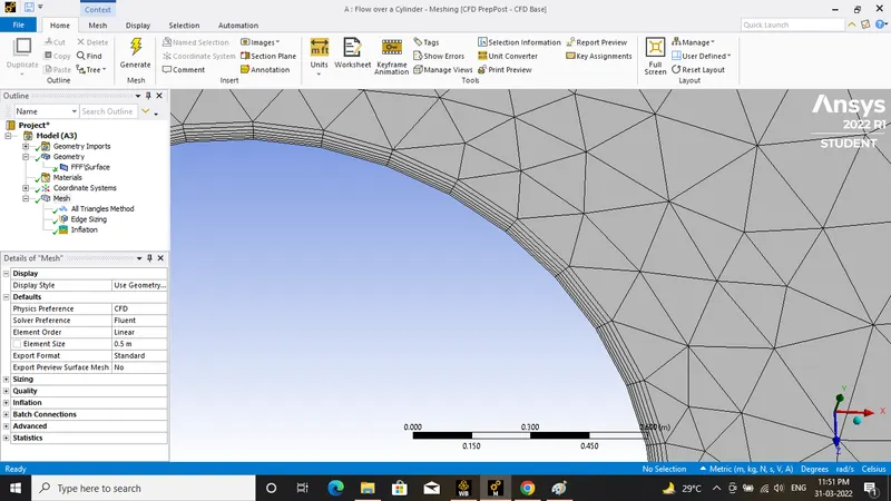
4.Then we should add inflation which is used to create a body-fitted mesh.

No.Inflationa Layers: 6

Launching Fluent:

Fluent details/Procedure:

• Use Laminar model

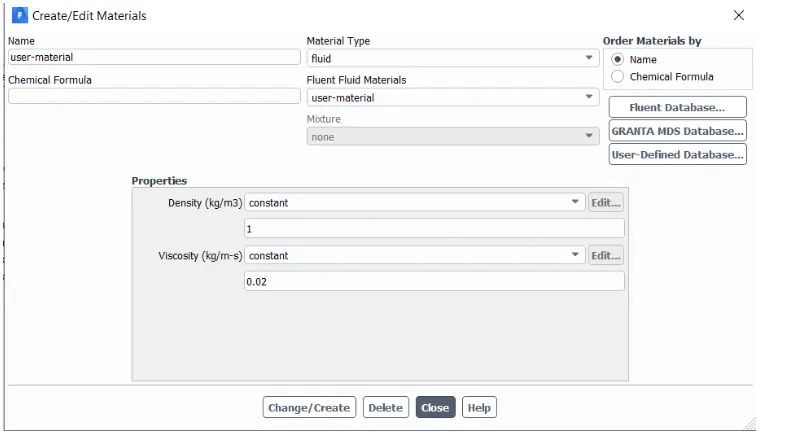
• Fluid: user-material

• Method of discretization: SIMPLE

• Density: 1

• Dynamic-viscosity: 0.02

• Creating a monitor point behind the cylinder by selecting points under surfaces.

• After creating the monitor point, create reports/plots for drag, lift velocity w.r.t cylinder or wall.

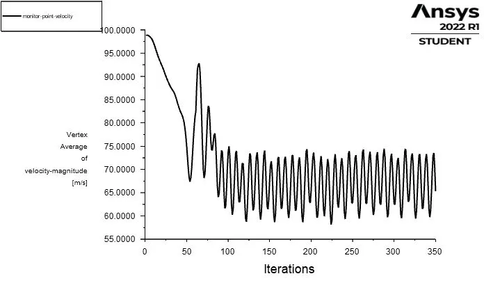
• Create plots for the velocity at the monitor point to analyze the vortex shedding.

• Use hybrid initialization for steady-state and standard for transient state (unsteady-state) simulations.

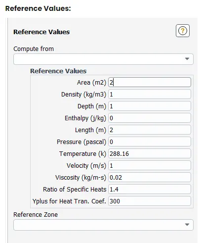
• Assign reference values repectively.

Part I:

Simulate the flow with the steady and unsteady case and calculate the Strouhal Number for Re= 100 and inlet velocity 1 m/s. Length 2 meter, Density 1 kg/m3, dymanic viscosity 0.02 kg/m-s

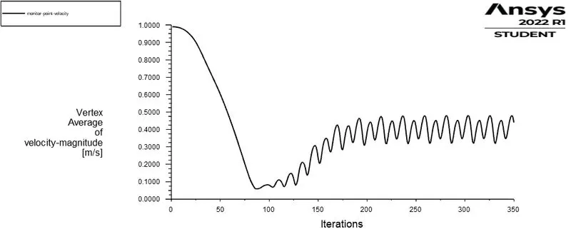
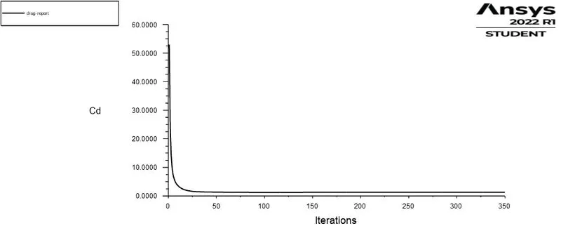
Steady-state: Re=100

Residuals:

Vertex average of velocity magnitude:

Drag plot:

Lift-plot:

Velocity-contour:

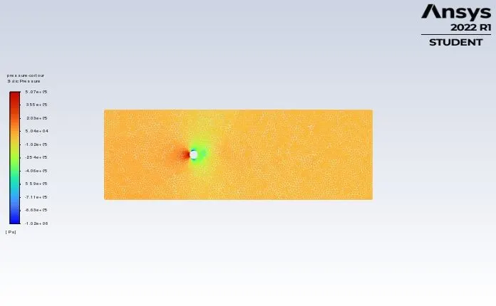
Pressure-contour:

Unstaedy state, Re=100

No of Time steps=1000 , Time step size=0.1

Residuals:

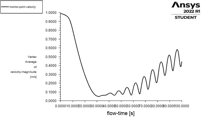
Vertex average of velocity magnitude:

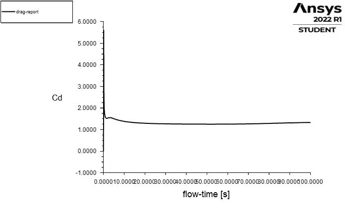
Drag-plot:

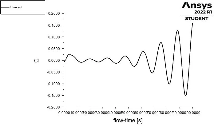
Lift-plot:

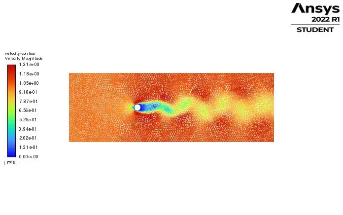
Velocity-contour:

Pressure-contour:

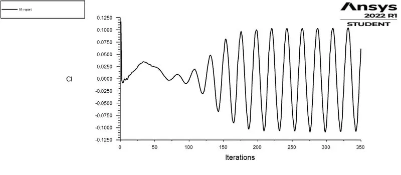
Frequency of Vortex Sheddinng:

f = Number of cycles/time of cycles

f = 0.08

Strouhal Number = (f * D)/ U

= (0.08 * 2)/1

= 0.16

---------------------------------------------------------------------------------------------------------------------------

PART-II

A] Simulating the flow with a steady-state solver for Re=10 and inlet velocity=0.1 m/s.

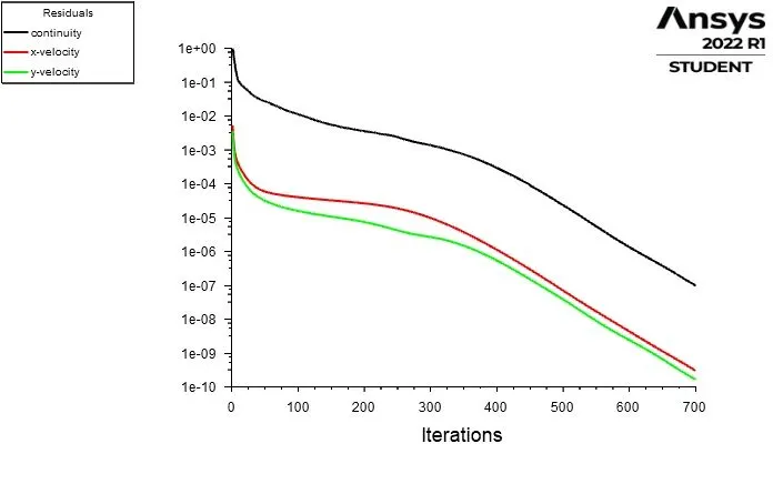
Residuals:

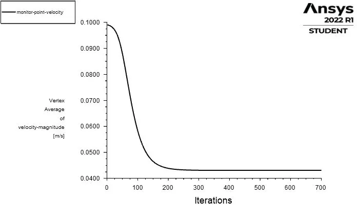
Vertex average of velocity magnitude:

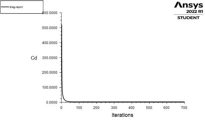
Drag-plot:

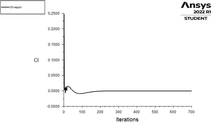
Lift-plot:

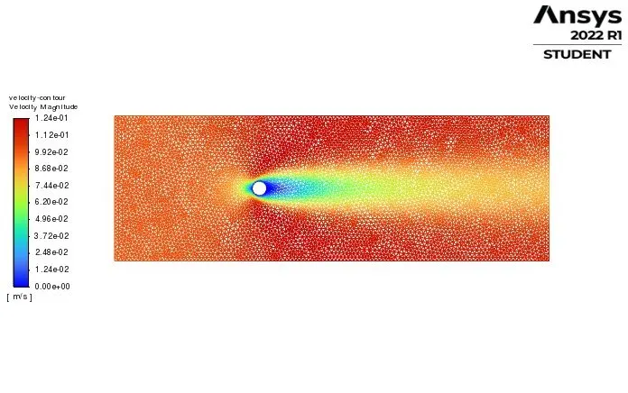
Velocity-contour:

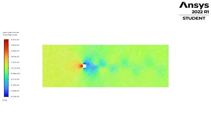
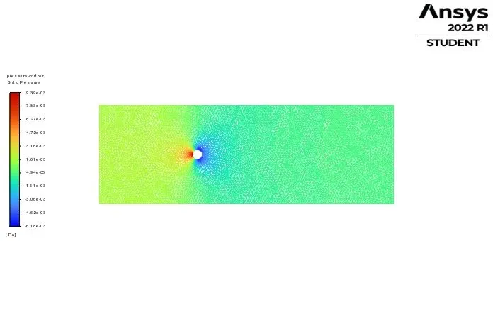
Pressure-contour:

B] Simulating the flow with a steady-state solver for Re=1000 and inlet velocity=10 m/s.

Residuals:

Vertex average of velocity magnitude:

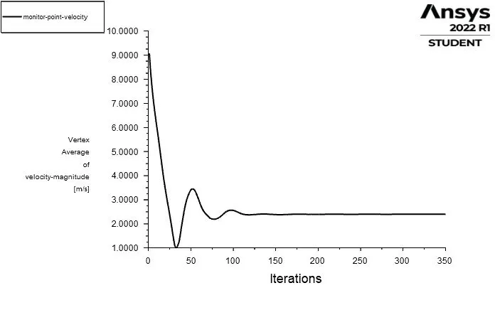
Drag-plot:

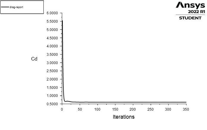
Lift-plot:

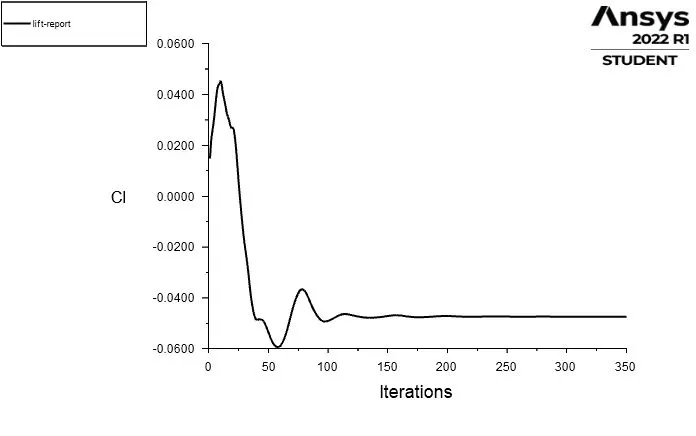
Velocity-contour:

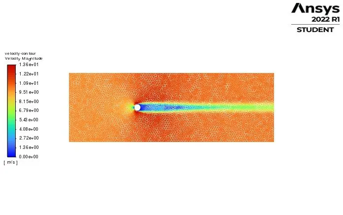
Pressure-contour:

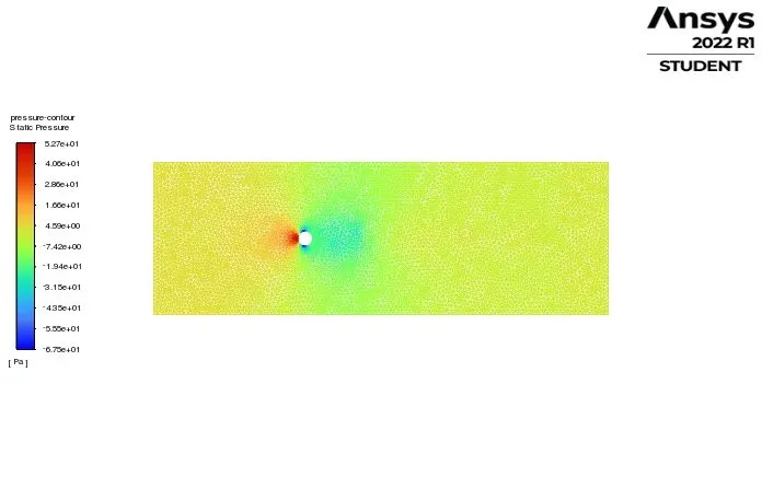
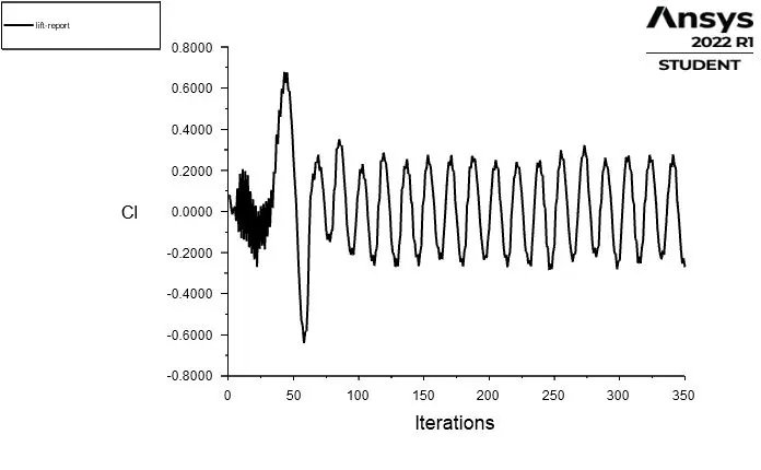
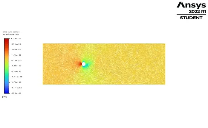
C] Simulating the flow with a steady-state solver for Re=10000 and inlet velocity=100 m/s.

Residuals:

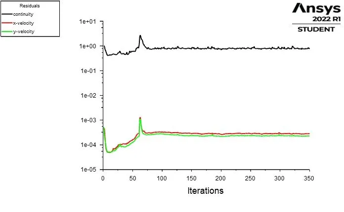
Vertex average of velocity magnitude:

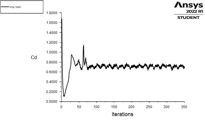
Drag-plot:

Lift-plot:

Velocity-contour:

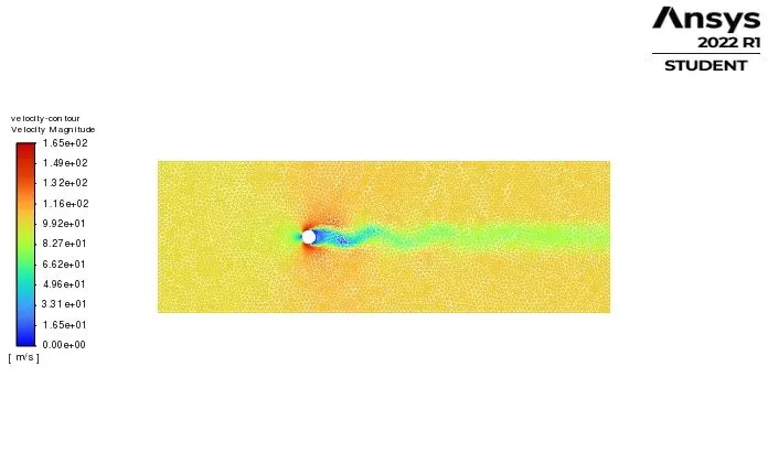
Pressure-contour:

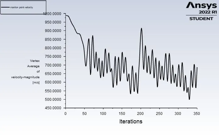
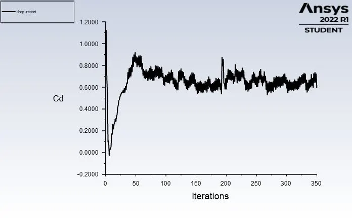
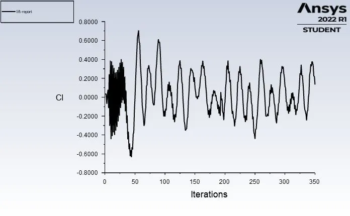
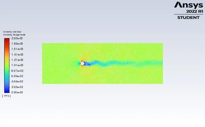
D] Simulating the flow with a steady-state solver for Re=100000 and inlet velocity=1000 m/s.

Residuals:

Vertex average of velocity magnitude:

Drag-plot:

Lift-plot:

Velocity-contour:

Pressure-contour:

Reynolds Number	Coefficient of Drag	Coefficient of Lift	Velocity
10 [steady state]	3.3138973	-0.000301668	0.1
100 [steady state]	1.3056	0.061355	1
100 [Unsteady state]	1.3312	0.15787	Time step=1000 Step size=0.1
1000 [steady state]	0.61095	-0.047369	10
10000 [steady state]	0.67785	-0.27047	100
100000 [steady state]	0.59202	0.1336	1000

Some Important Points to be noted:-

1. In Fluent you can get animations for both steady state and transient state problems.
2. In CFD posts you can get animations for steady state in Quick animation and Keyframe animation.
3. Timestep animation in CFD-Post is suitable for transient problems.
4. When the reynolds number increases the coeffecient of drag decreases. Moreover, when the reynolds number is large (Re>4000) flow will be turbulent( Chaotic and swirling vortices), in which laminar flow is very small and which leads to lower skin friction drag.
5. Firstly , when the velocity increases coeffecient of drag decreases.
6. Secondly, for the reynolds number 100 vortices can be seen because of low velocity and only boundary layer seperation occured.Also, in low reynolds number coeffecient of drag increases.
7. For the steady case the flow is not dependent on time step so strouhal number cannot be calculated for the steady state but the solution has reached the steady state after some iterations. We can see vortices for higher reynolds number only.
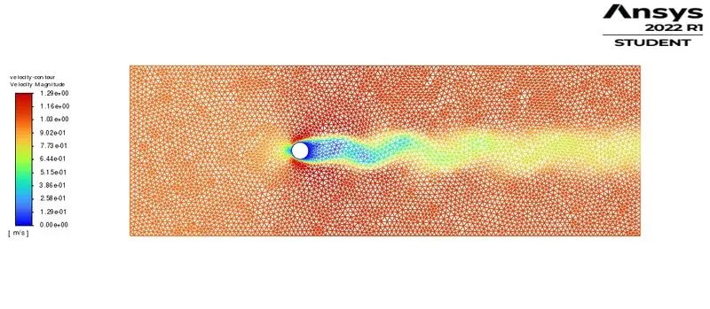
8. For better visualization we can use contour, vector and streamline to see the vortex generation when the flow past over a cylinder.
9. For reynolds number 100 ( Unsteady state) the vortices can be seen and the shedding frequency calculated.In addition, the value of 0.16 strouhal number is calculated.
10. In this case the boundary layer seperation decreases there will be less recirculation flow at wake region behind the cylinder with the reduced drag.For all the simulation parameters are kept constant except for the velocity, so increasing the velocity will increase reynolds number.
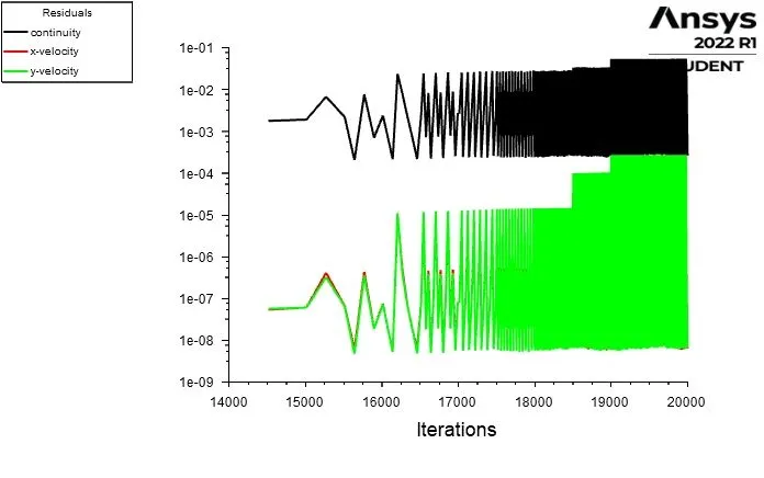
11. In transient case lift coeffecient keeps on changing beacuse of alternate nature of the vortices it never settle down and keeps on repeating same pattern after some iteration( residual plot).When it comes to steady case the flow is not dependent time so the lift coeffecient becomes constant after some iterations.
12. Among various flow regimes observed, Negative values of lift coefficient are found to be occure only at low angles of attack. Which is corresponds to laminar separation without floe transition and without reattachment.