Week 2 - Flow over a Cylinder.

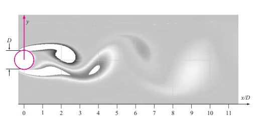
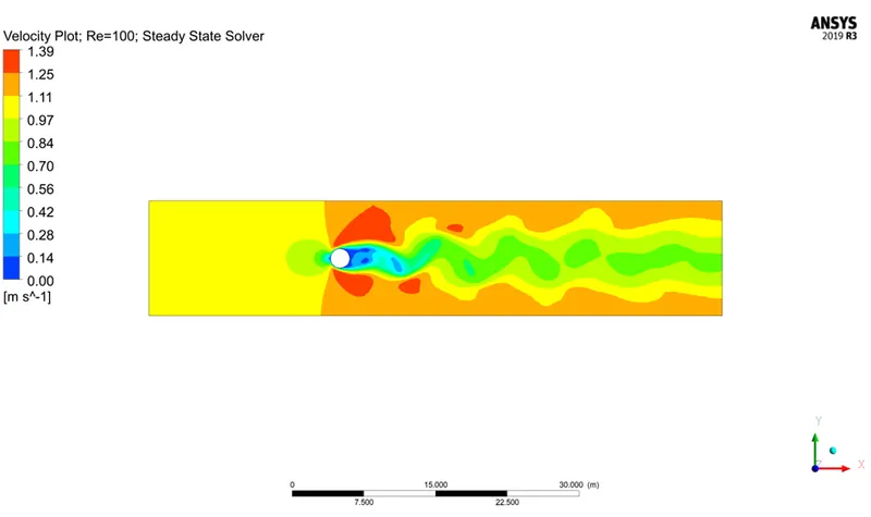
Whenever a body moves through a medium of fluid or when the fluid is made to flow over the body, the body experiences at least a base level drag force which is especially due to the formation of a vacuity region followed by the formation of swirls/ eddies/ vortices behind the body. These vortices are created by the mixing of two separate streaklines from the top and bottom getting closer due to pressure difference caused by the void and eventually forming large vortices. This phenomenon of forming a large number of vortices is called Karman Vortex Street. These are the most spectacular and fascinating patterns created by the shear flow. It is a rotary flow about an axis and has no radial velocity component. These have low pressure at the centers of the vortices.

Here is the picture depicted below which picturizes the flow over the cylinder(2-D) of 1-meter diameter and the flow velocity is estimated to be around 0.00219 m/s with a Reynolds number of 150 for the medium of air at 15^oC (Reference: Fluid Mechanics Fundamentals and Applications)

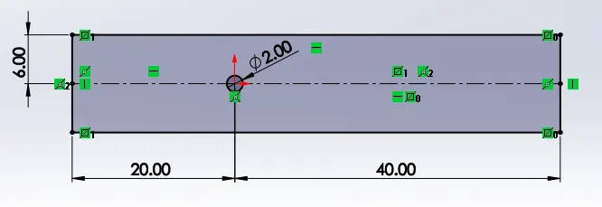
Outline Geometry:

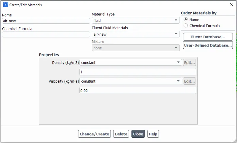
The outline of the geometry which we need to analyze is given below with a cylinder of diameter 2 meters over which the flow at a necessary Reynolds number of 10, 100, 1000, 10000 and, 100000 is made by varying the velocity and by fixing the assumed values of density and viscosity to be 1 Kg/m³ and 0.02 Ns/m².

x-Velocity values for varying Reynolds numbers:

Reynolds Number	Velocity(m/s) [Density:1 Kg/m3 ; Viscosity:0.02 Ns/m2]
10	0.1
100	1
1000	10
10000	100
100000	1000

The solving methods of both steady and transient states are implemented for the flow condition of Re=100, and the remaining are analyzed with the steady-state conditions.

Process using ANSYS FLUENT:

1.SpaceClaim:

The first step is to create the geometry for the simulation similar to the one which is shown above using Ansys SpaceClaim.

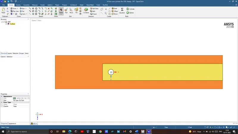
Here, two rectangular regions are created, where the yellow region is much essential to capture the vortex shedding, thus we control the mesh size over there effectively and the orange portion can be filled with elementary mesh size thus making the overall computing time lesser. The below image shows the meshed geometry of the above one.

2. Ansys Mechanical(Pre-Post):

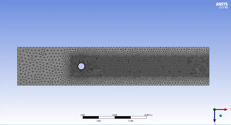
The various mesh optimization techniques used were, using the Triangular mesh method, Face sizing(Outer{1 meter} & Inner Rectangles{0.25 meters}), Edge sizing(Inner cylinder wall{36 Divisions}), and Inflation(to capture the Boundary layer separation near the cylinder wall{8 Layers; First Layer Thickness: 5e-3 meters; Increment Rate: 1.2}). And we eventually name the boundaries as inlet, outlet, symmetry, and wall. Then we open up the Fluent Software with a parallel simulation method to initiate and run the simulation.

3. Ansys Fluent:

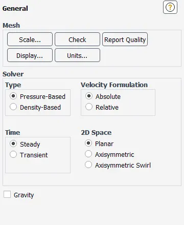
• The General Settings include the indication of the Solver type(Pressure/Density-based) for which we go with Pressure-based solver since the flow is considered to be a subsonic and Velocity Formulation(Absolute/Relative) fo which we go with the Absolute Velocity Formulation type. And based on the type of Solving, we choose either Steady(Iteration based) or Transient(Time-Step based).
• Then the material properties are given using create material, by creating an imaginary fluid which is termed by us as air-new and thus deleting the original air-fluid properties.
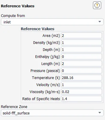
• Then the Reference values are entered according to the cylinder geometry(Area[Projected]:2m²; Depth: 1m[Default for any 2-D system]; Characteristic Length: 2m), from the Inlet.

• Then another important parameter is to fix the Solution Methods. The scheme that we use here is SIMPLE and some discretization methods were set.

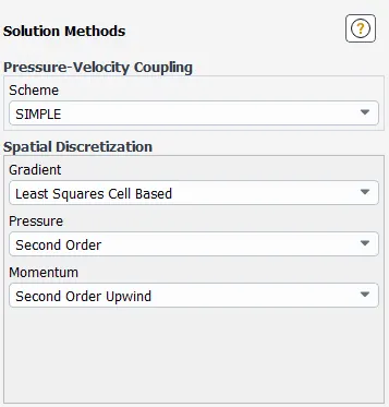
• Then eventually set up the monitor point 6 meters behind the wall, and define a plot of Vertex average velocity w.r.t Iterations at that monitor point, and then initialize the solution with the hybrid method.
• Create plot definitions for Drag Coefficient and Lift Coefficient for the wall and also create a contour plot for velocity and include that in animation to view the periodic variation of it over time.
• And at last, Run the simulation by giving the No. of Iterations for Steady-State Solver or a number of time-steps and time-step size and Iterations per time step for Transient-State Solver.

Strouhal Number: Each bluff body shape has a particular(Strouhal number) value depending on characteristics of the flow separation. For example: If the diameter of a circular cylinder is increased keeping the velocity constant, the vortex shedding frequency will decrease. Similarly, an increase in the velocity will increase the vortex shedding frequency and vice versa.

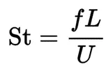
Here the term f represents the frequency or Number of peaks per-flow time, L represents the characteristic length of the body, and U represents the outer velocity of the fluid. Strouhal number is a dimensionless entity.

PART-I:

Here we simulate the flow with the steady and unsteady case and calculate the Strouhal Number for Re= 100.

Reynolds Number= 100:

Steady State Solver:

Velocity Plot:

Residual Plot:

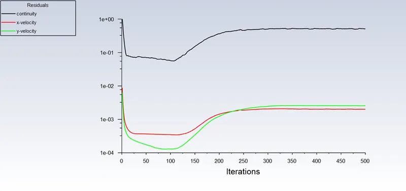
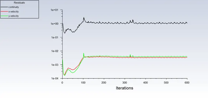
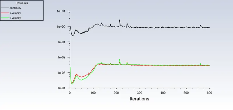
The Residual plot shows the convergence of the solution which conveys us the end result for that simulation.

Monitor Point Velocity:

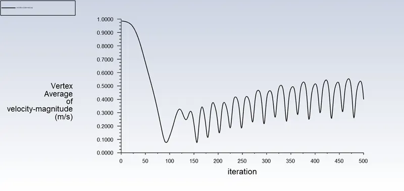
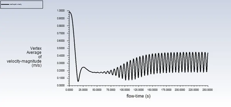
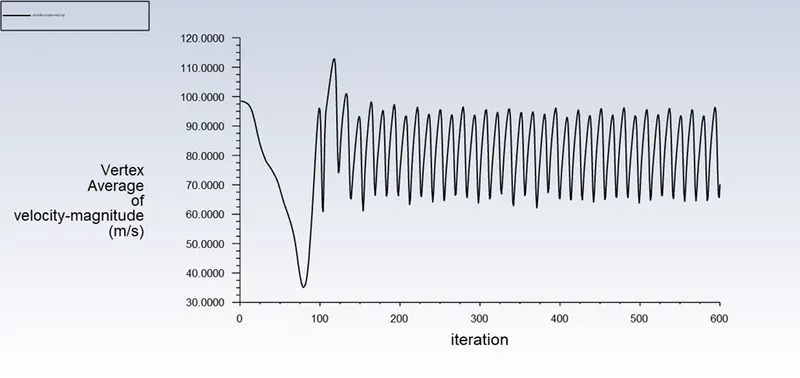
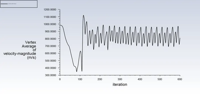
The fluctuation in the monitor point velocity is due to the formation of vortices behind the cylinder.

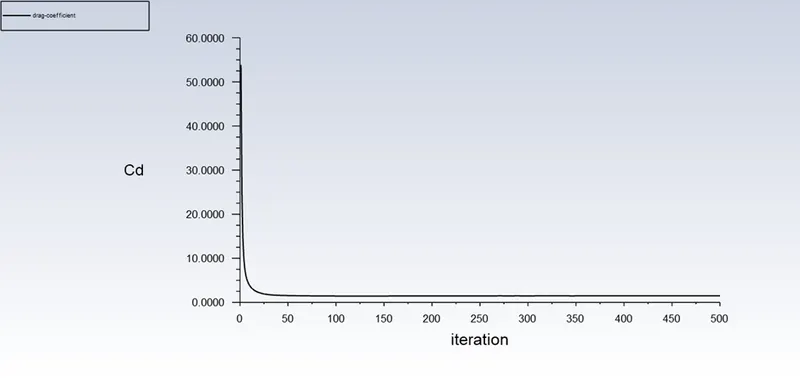
Coefficient of Drag:

Coefficient of Lift:

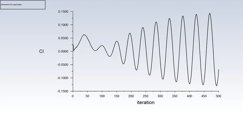
Strohal number(From Lift Force Plot):

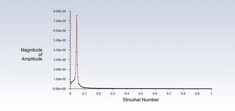
The Strouhal number for this criteria is obtained as (0.04-0.05).

Transient State Solver:

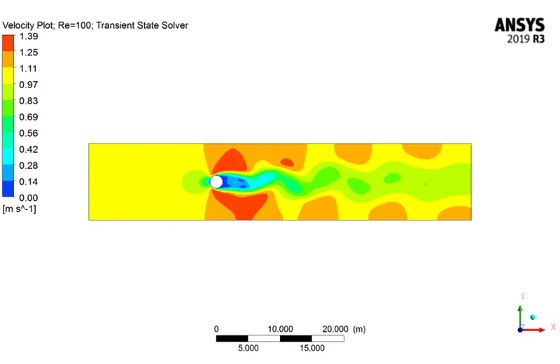
The transient simulation was run for the time-step size of 0.25 seconds so that the optimal solution was obtained without any numerical disruption due to the Courant number.

Velocity Plot:

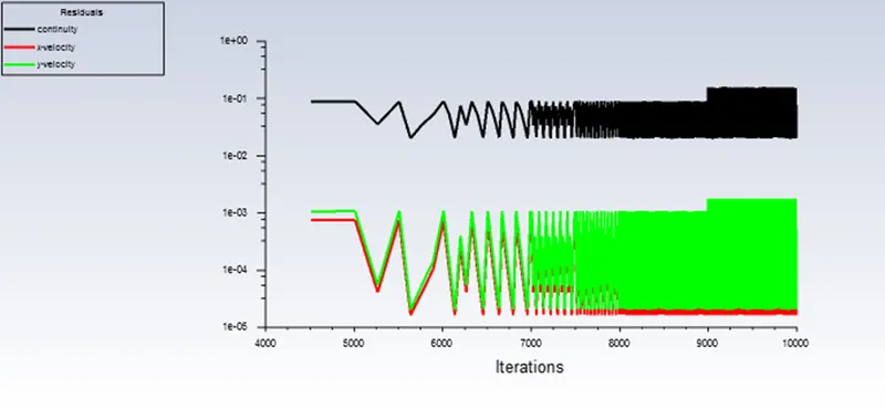
Residual Plot:

Monitor Point Velocity Plot:

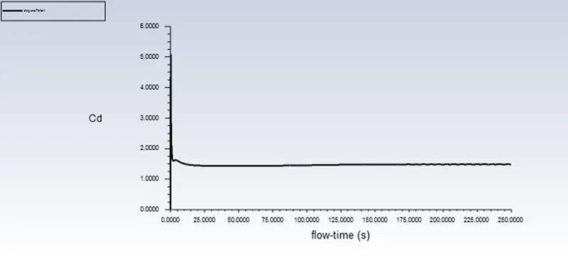
Coefficient of Drag Plot:

Coefficient of Lift Plot:

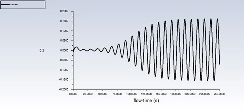
Strohal number(From Lift Force Plot):

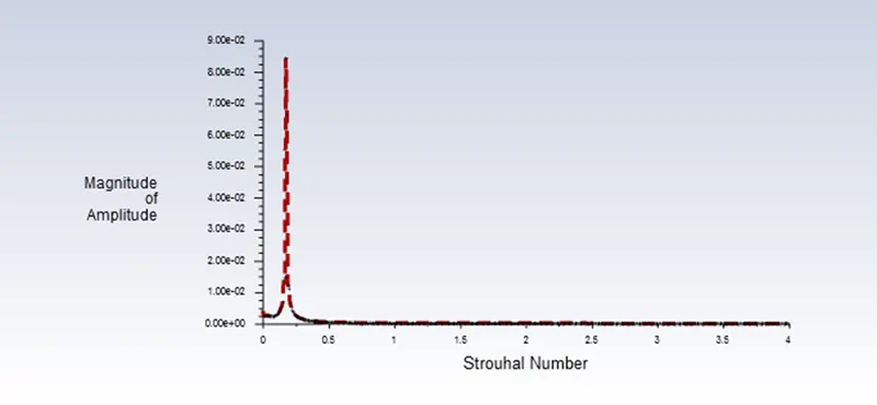
The Strouhal number for this criteria is obtained as (0.03-0.04).

The comparison of Strouhal numbers for different types of solvers is made below.

Solver Type	Strouhal Number
Steady State	0.04-0.05
Transient State	0.03-0.04

PART-II:

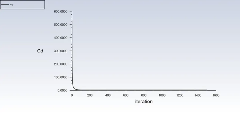
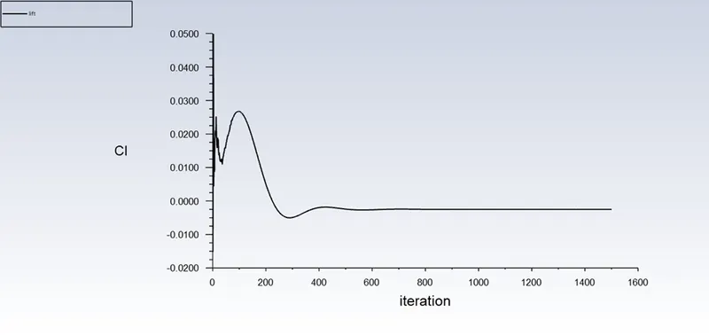
Here we calculate the coefficient of drag and lift over a cylinder by setting the Reynolds number to 10,1000,10000 & 100000 and we run with a steady-state solver.

Reynolds Number= 10:

Steady State Solver:

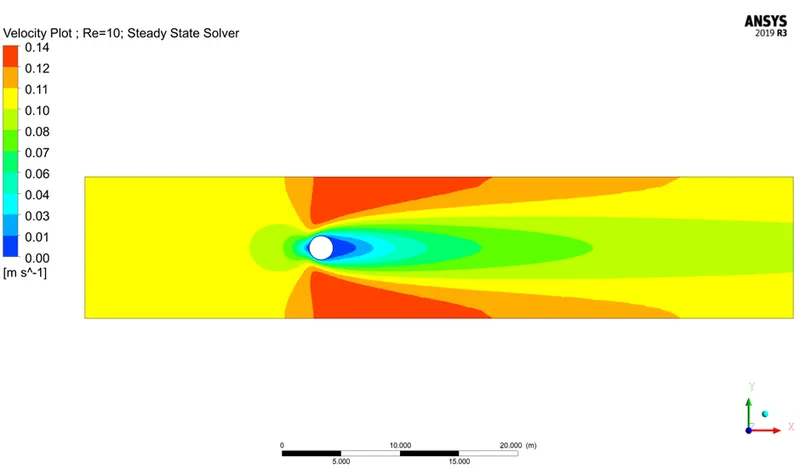
Velocity Plot:

Here the pure laminar flow(Re=10) gives a smooth transition across the cylinder and doesn't have enough momentum for dissipation to form the corresponding vortices. Thus it has the largest drag force of any flow cases studied by us.

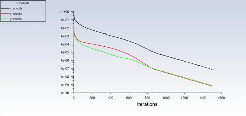
Residual Plot:

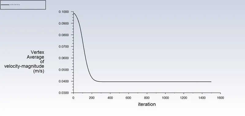
Monitor Point Velocity Plot:

Coefficient of Drag Plot:

Coefficient of Lift Plot:

Strohal number(From Lift Force Plot):

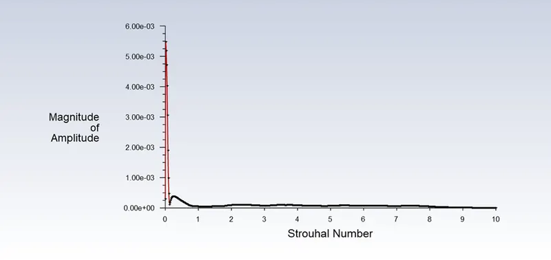
The Strouhal number for this criteria is obtained as around 0.01.

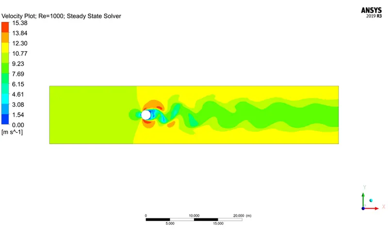
Reynolds Number= 1000:

Steady State Solver:

Velocity Plot:

Residual Plot:

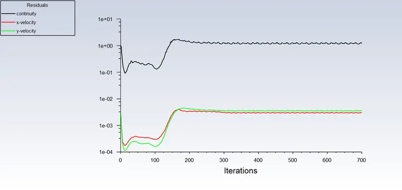
Monitor Point Velocity Plot:

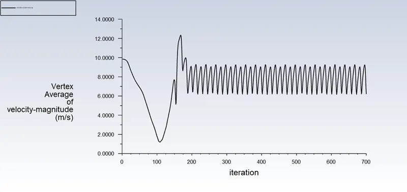
Coefficient of Drag Plot:

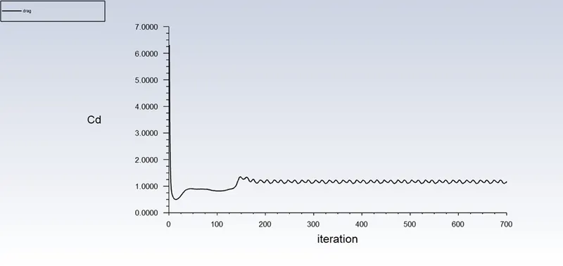
Coefficient of Lift Plot:

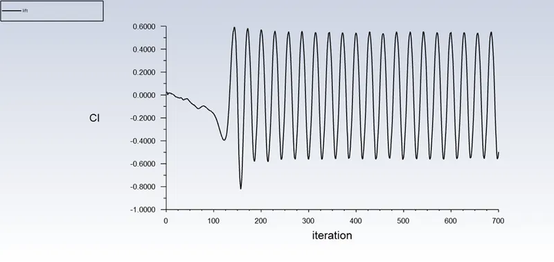
Strohal number(From Lift Force Plot):

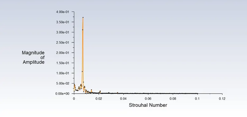
The Strouhal number for this criteria is obtained as (0.009-0.01).

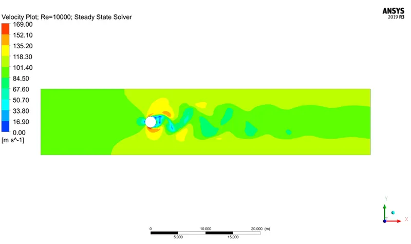
Reynolds Number= 10000:

Steady State Solver:

Velocity Plot:

Residual Plot:

Monitor Point Velocity Plot:

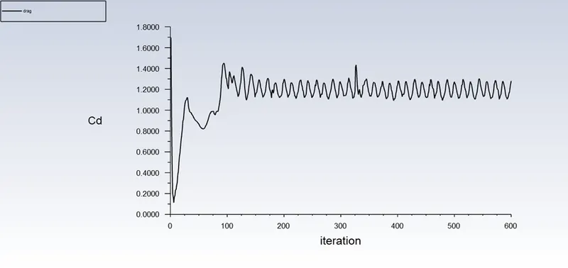
Coefficient of Drag Plot:

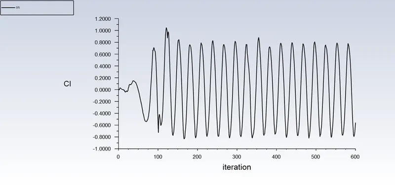
Coefficient of Lift Plot:

Strohal number(From Lift Force Plot):

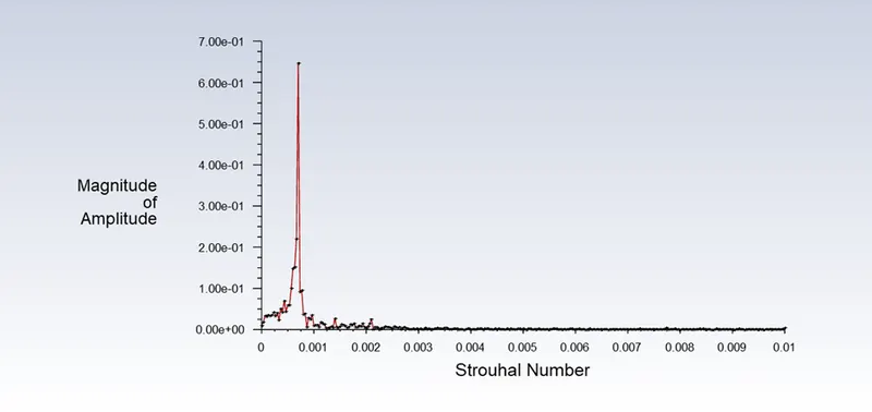
The Strouhal number for this criteria is obtained as 0.0009.

Reynolds Number= 100000:

Steady State Solver:

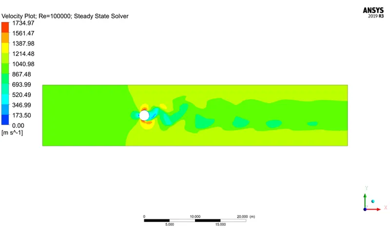
Velocity Plot:

Residual Plot:

Monitor Point Velocity Plot:

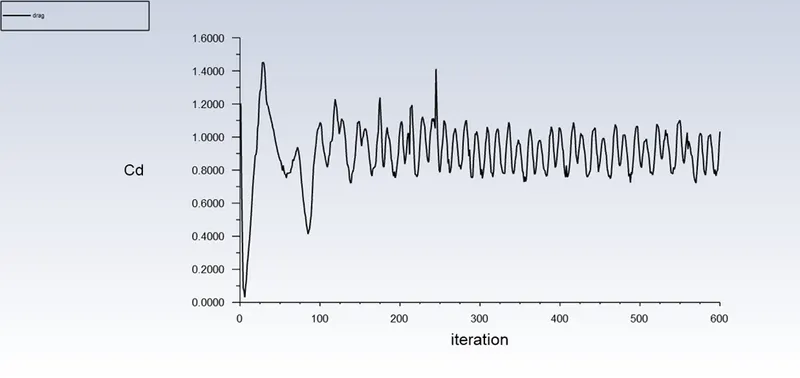
Coefficient of Drag Plot:

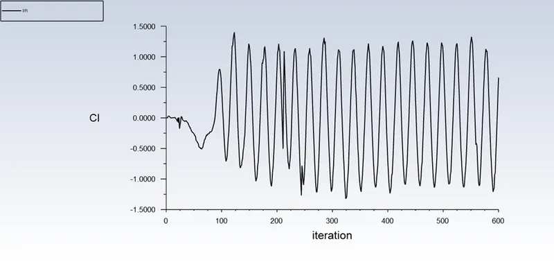
Coefficient of Lift Plot:

Strohal number(From Lift Force Plot):

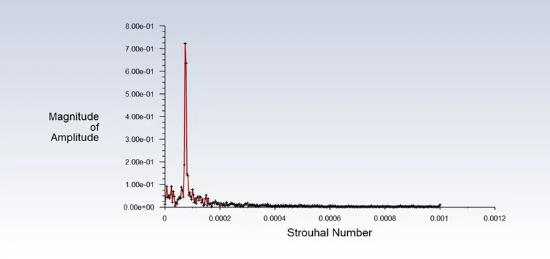
The Strouhal number for this criteria is obtained as 0.0001

Drag Force Coefficient Comparison:

Reynolds Number	Drag Force Coefficient
10(Steady)	3.9181
100(Steady)	1.5001
100(Transient)	1.479
1000(Steady)	1.1775
10000(Steady)	1.2805
100000(Steady)	1.0328

It seems that as the Reynolds number increases the Drag force coefficient eventually decreases. This is due to the momentum dissipation and vortex formation property of the high Reynolds number flows.

This is evident from the Journal which is given through the link here: https://drive.google.com/file/d/1ezwJZhxMKKcQ6Tl19tKyuY8pgGLk5Ky8/view?usp=sharing

Referred Book: Fluid Mechanics Fundamentals and Applications