Flow over a Cylinder.

AIM:

PART 1

1. Simulate the flow over the steady and unsteady case and calculate the Strouhal number for Re=100.

PART 2

1. Calculate the coefficient of drag and lift over a cylinder by setting the Reynolds number to 10,100,1000,10000 & 100000 (Run with steady solver).

2. Discuss the effect of Reynolds number on the coefficient of drag. [ Results should be validated with any standard literature and error should be within 5%].

Expected results:-

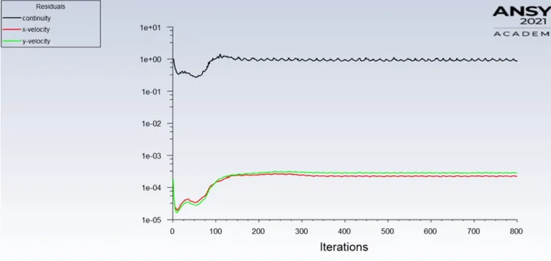
1. In both approaches, show that the flow has converged. That is, what quantities or plots need to be looked at to determine that the flow has converged?
2. Plots of the coefficient of drag and lift.
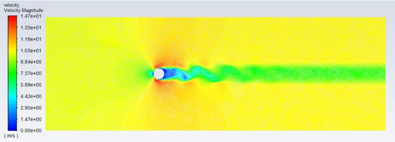
3. Plots to show vortex shedding behind the cylinder.

INTRODUCTION

Vortex Shedding: Vortex Shedding is an oscillatory flow that takes place when a fluid flows past a bluff body at a certain velocity depending upon the size and shape of the body. In the flow, vortices are created at the back of the body and detach periodically from either side of the body forming the Von Karman Vortex Street. The fluid flow past the object creates alternating low-pressure vortices on the downstream side of the object. The object will tend to move toward the low-pressure zone. In spite of extensive experimental and numerical studies almost over a century, flow around a circular cylinder still remains a challenging problem in fluid mechanics, where intensive investigations are continued even today to understand the complex unsteady dynamics of the cylinder wake flow.

Governing Equations

The frequency at which vortex shedding takes place for an infinite cylinder is related to the Strouhal number by the following equation:

Where is the dimensionless Strouhal number, is the vortex shedding frequency (s^-1), is the diameter of the cylinder (m) and is the flow velocity (m s^-1).

The Strouhal number depends on the Reynolds number , but a value of 0.22 is commonly used. Over four orders of magnitude in Reynolds number, from 100 to 100000, the Strouhal number varies only between 0.18 and 0.22.

Co-efficient of drag `Cd`: In fluid dynamics, the drag coefficient (Cd) is a dimensionless quantity that is used to quantify the drag or resistance of an object in a fluid environment, such as air or water. It is used in the drag equation in which a lower drag coefficient indicates the object will have a less aerodynamic or hydrodynamic drag. The drag coefficient is always associated with a particular surface area.

The drag coefficient of any object comprises the effects of the two basic contributors to fluid dynamic drag: skin friction and form drag. The drag coefficient of a lifting airfoil or hydrofoil also includes the effects of lift-induced drag. The drag coefficient of a complete structure such as an aircraft also includes the effects of interference drag. The drag coefficient Cd is defined as

`Cd=(2⋅Fd)/(ρu^2A)`

where: Fd is the drag force, which is by definition the force component in the direction of the flow velocity,

ρ is the mass density of the fluid,

u is the flow speed of the object relative to the fluid,

A is the reference area.

Co-efficient of lift `CL`: The lift coefficient (CL) is a dimensionless coefficient that relates the lift generated by a lifting body to the fluid density around the body, the fluid velocity, and an associated reference area. A lifting body is a foil or a complete foil-bearing body such as a fixed-wing aircraft. CL is a function of the angle of the body to the flow, its Reynolds number, and its Mach number. The section lift coefficient cl refers to the dynamic lift characteristics of a two-dimensional foil section, with the reference area replaced by the foil chord.

`CL=(2L)/(rhou^2S)`

where L, is the lift force,

S is the relevant surface area and

q is the fluid dynamic pressure, in turn, linked to the fluid density, and to the flow speed.

Procedure: Geometry

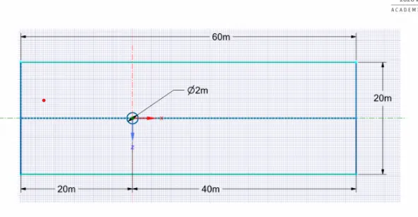
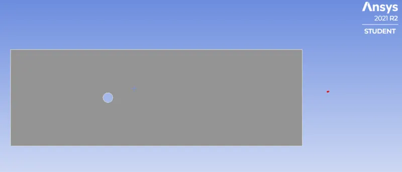
An infinitely long circular cylinder of diameter D=2.0 m is placed in an otherwise undisturbed uniform crossflow. The lateral boundary and the exit boundary in the far wake are placed at 10 D and 20D from the center of the circular cylinder, respectively. The cylinder is used to be drawn in SpaceClaim.

Meshing

1. Select the faces and create named selections for easy application of boundary conditions as inlet, outlet, walls and symmetry.

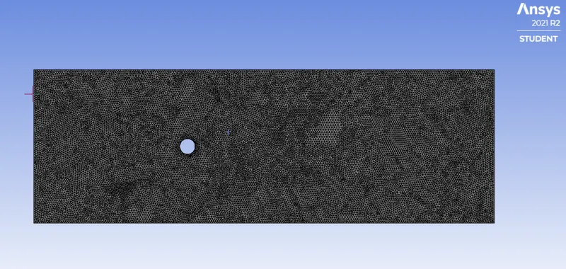
2. Mesh size is 0.25m and mesh type is triangular(change it in the mesh-type) it has not defaulted.

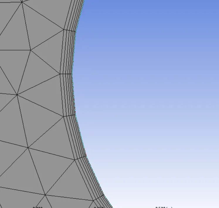
3)Apply inflation for better capturing of physics near-wall of the cylinder, 6 inflation layers with 0.005m.

Solving :

1. select laminar flow inside the viscous model.

2. As we wanted to customize material property for simulation, go to materials > fluent database > select the material (air) > copy it> rename the name of the material.

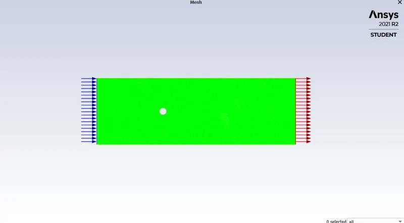
Boundary Condition:

Outlet : gauge pressure = 0 Pa.

wall: no-slip condition.

SIMPLE algorithm with the laminar viscous model is used in a steady-state analysis.

plots: In both i.e. steady and unsteady state simulations, the following plots are to be shown:

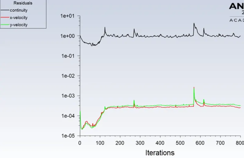
Residual plot - This plot helps us in knowing at what point convergence is achieved.

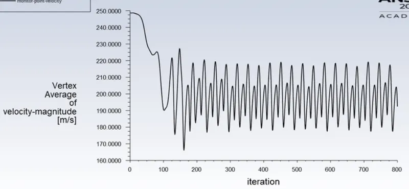
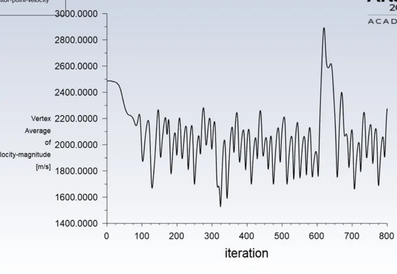
Monitor point velocity plot - A monitor point is placed at a distance of 8m from the cylinder in order to calculate the velocity at that point.

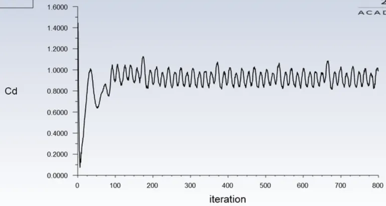
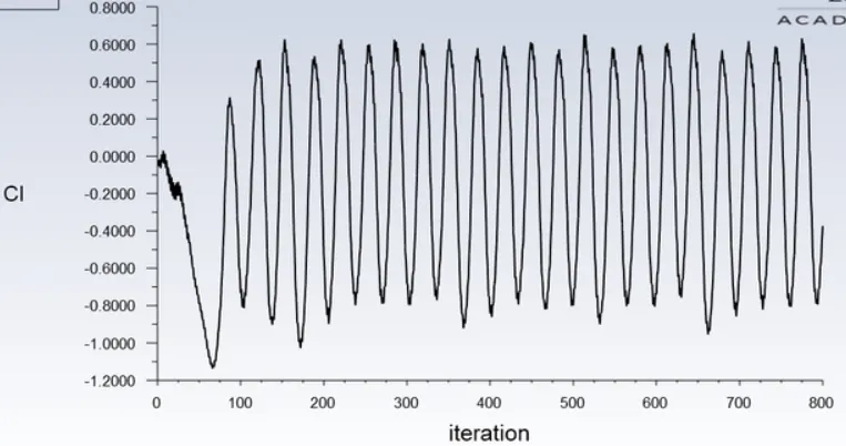
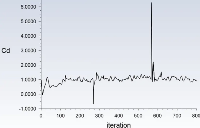
Drag coefficient plot - To calculate the drag coefficient.

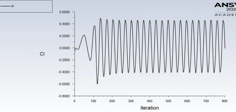
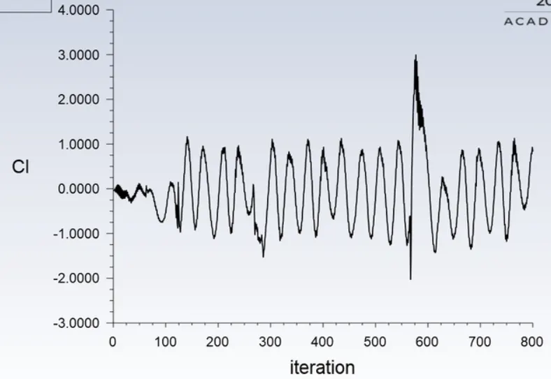
Lift coefficient plot - To calculate the lift coefficient.

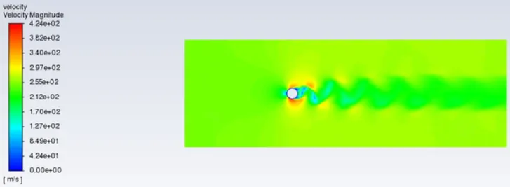
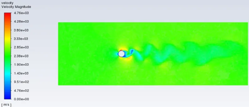
Velocity contour plot - To see the velocity changes in the flow over the cylinder.

For RE=10

Steady-state analysis

v=0.25m/s

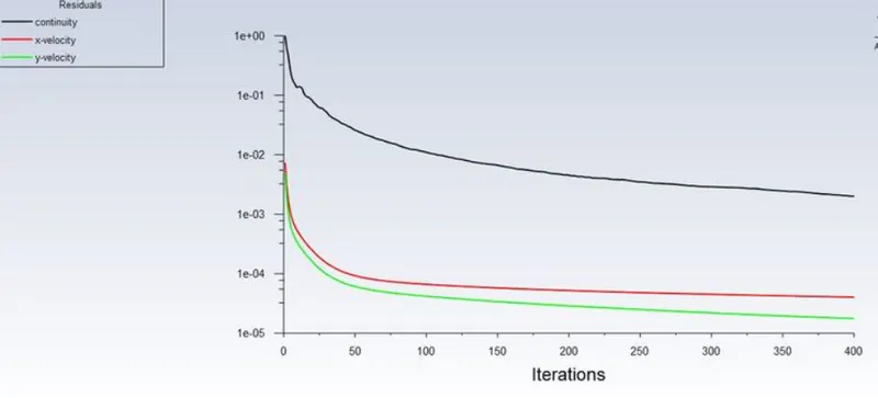
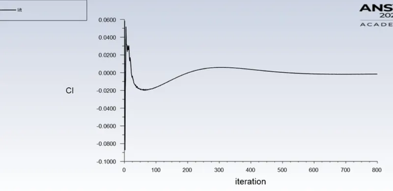
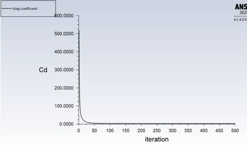
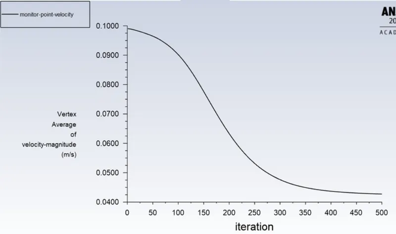
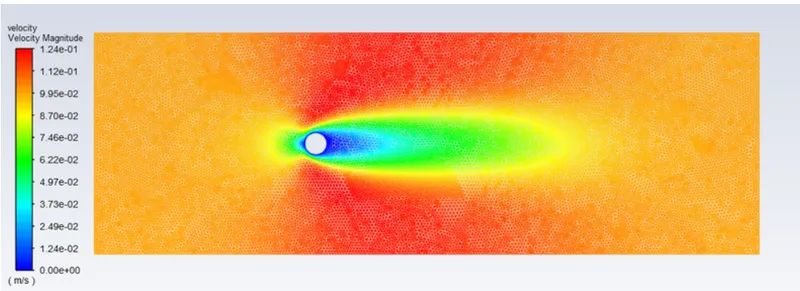
No vortex shedding is observed with Re=10.

FOR RE=100

velocity=2.5m/s

steady-state solver

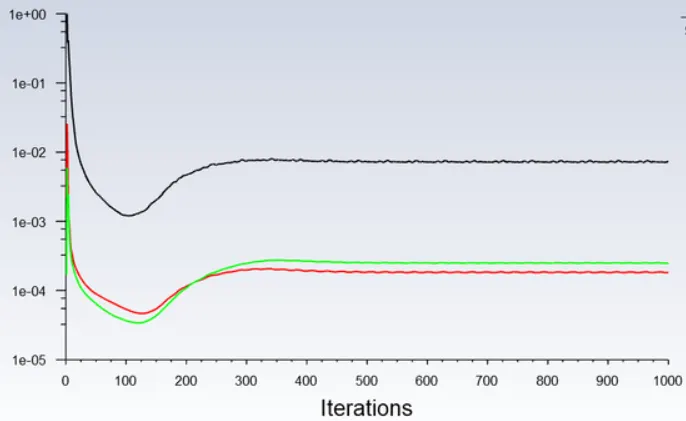
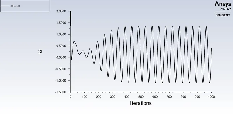
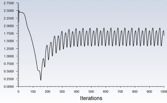
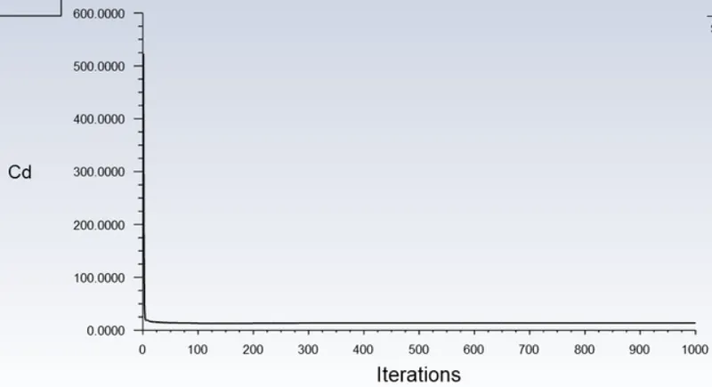
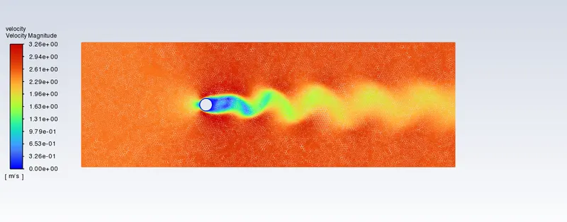
FOR RE=100

velocity=2.5m/s

unsteady-state solver

SIMPLE-C algorithm is used with time step size=1

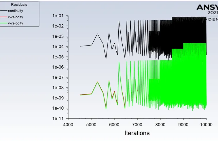
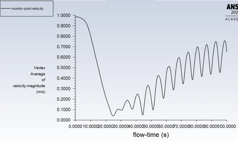
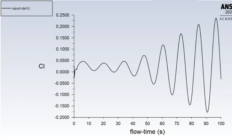
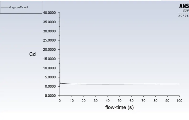
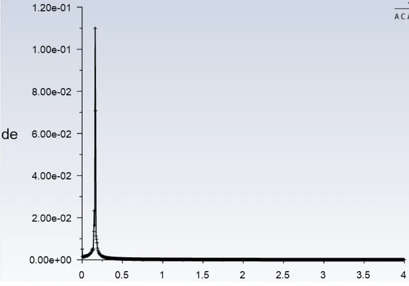
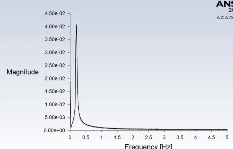
By opening the FFT file in excel, the max Strouhal number value is found to be 0.112.

Reynolds number: 1000

Velocity: 25

viscosity : 0.05

Iterations: 1000

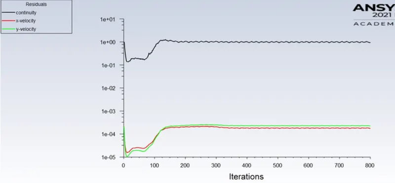
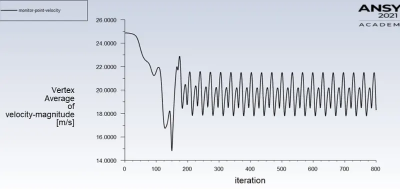
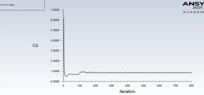
Reynolds number = 10000.

velocity = 250 m/s.

density = 1 kg/m3.

viscosity = 0.05 Pa-s.

Reynolds number = 100000.

velocity = 2500 m/s.

density = 1 kg/m3.

viscosity = 0.05 Pa-s.

Results

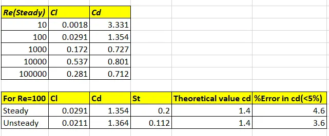
In the first case, the flow over a cylinder is simulated for both Steady and unsteady cases with Re=100, and with the results generated the phenomena of Von Karman Vortex Street are also observed. Necessary plots are plotted in order to observe that the flow is converged and the vortex shedding is happening. Contours are generated in order to observe the flow over a cylinder. By plotting Power Spectral Density vs Frequency, the Strouhal number is calculated.

In the second case, six different simulations i.e (Re = 10,100,1000,10000,100000,1000000) are simulated to observe the behavior of the drag and lift coefficients by changing the Reynolds number. In order to observe the behavior of the drag coefficients for the simulations, the velocity of the flow is varied to change the Reynolds number and the rest of the parameters are kept constant. As we know if the Reynold number is less than 2000, then flow in a pipe is Laminar. Hence we use the Viscous model = Laminar. For Re=10, it is observed that there is no formation of vortex shedding and in the rest of the cases, it is clearly observed. As per the basic conditions and parameters, the results are validated from the literature. As we refine the mesh we need to run more iterations. From the above table, it can be concluded that the error percentage is less than 5%.

Reference Research Paper:- https://www.sciencedirect.com/science/article/pii/S0307904X08000243