Week 2 - Flow over a Cylinder.
Aim: - To simulate the flow over a cylinder and explain the phenomenon of Karman vortex street.
Objective: -
- To setup case for steady and transient simulation.
- To calculate the coefficient of drag and lift over a cylinder by setting different Reynolds numbers.
- To observe the effect of Reynolds number on coefficient of drag.
- To calculate the Strouhal number.
Theory
A very interesting sequence of events begins to develop when the Reynolds number is increased beyond 40, at which the wake behind the cylinder becomes unstable. The wakes develop a slow oscillation in which the velocity is periodic in time and downstream direction. The oscillation wake rolls up into two staggered rows of vortices with opposite sense of rotation. And these rows form a street known as von Karman vortex street.
The Reynolds number is a key parameter in fluid dynamics. It describes the fluid, geometry and flow. This allows us to compare different fluid system.
`Re=[ρvD]/μ`
`ρ=` density of fluid
V = in flow velocity
D = diameter of cylinder
`μ=` dynamic viscosity of fluid
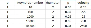
calculation of velocity for given Reynolds number in excel
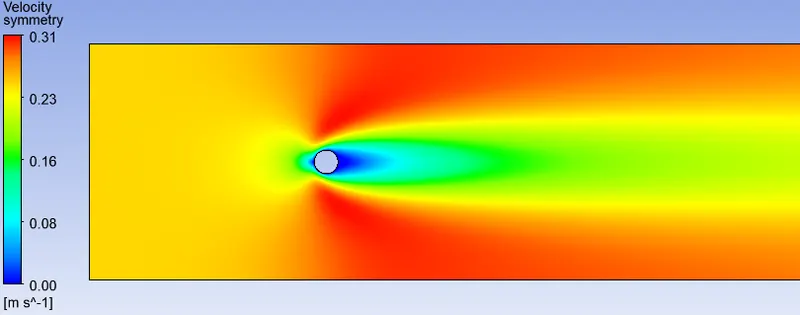
As we increase the flow rate or Re the flow develops into a variety of structures
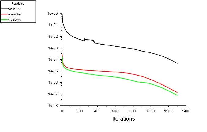
For Re = 10
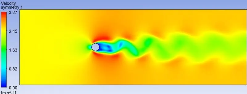
For Re = 100
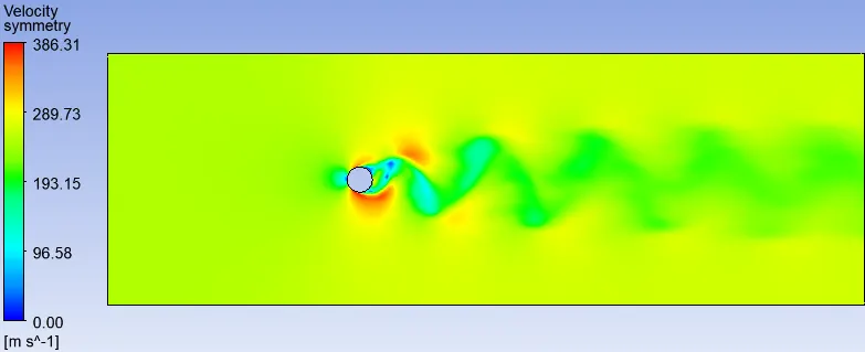
For Re = 1000
For Re = 10000
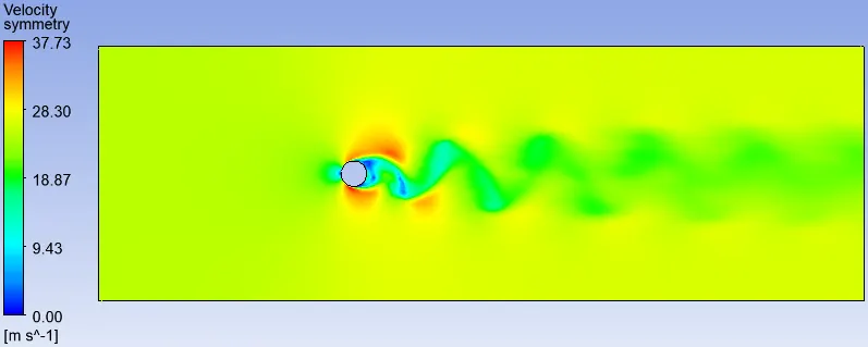
for Re = 100000
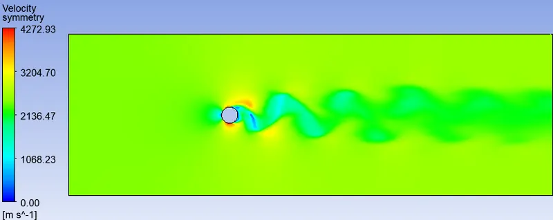
The flow is unstable resulting in a moving wake this increases the drag.
Near the wall pressure increases as the wall falls away this pushes the fluid back. Which causes change in direction of the fluid flow path. If the momentum is insufficient, the fluid reverses and separates from the wall the separation of the boundary layer can distinguish the wake. The further upstream separation occurs, the more drag is experienced by the cylinder.
solving and modelling approach
The main aim of the project is to study the behavior of Reynolds number on the flow over a cylinder. to capture the flow with every regime it is important to have more flow domain and less mesh size to capture every possible vortex in wake region.
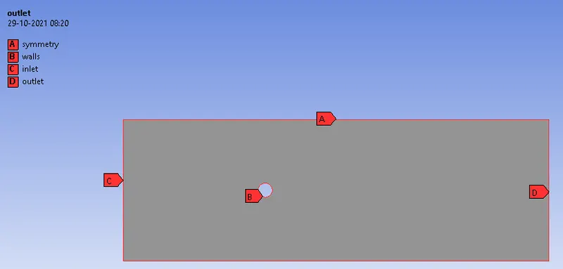
The problem is divided into two group in which both steady and unsteady state simulation will be carried accordingly. In steady state simulation the varying Reynolds number will be taken into consideration by maintaining fluid property constant. The simulation will be running for 10, 100, 1000, 10000, 100000 Reynolds number and accordingly the other parameters will be studied. The problem will start with 2D geometry of flow field and mesh afterwards. It is important to have less mesh size to capture every little detail from flow domain. The inflation layer will be added near the cylinder wall to capture the boundary layer detachment from the surface of cylinder. The boundary conditions will be simple as velocity inlet and pressure outlet with symmetry wall type condition. The cylinder will be also considering as wall type in which coefficient of lift and drag will be calculated.
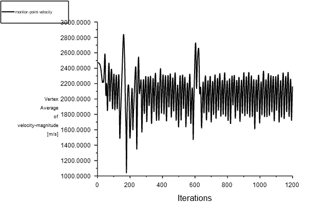
For steady state solver simple interpolation scheme will be used to calculate results in neighboring volume. Unsteady state simulation will also be done using the simple interpolation scheme. To check for convergence of solution. we will create some plots which have vertex average velocity 8m behind the cylinder which will be used to plot Strouhal number later using FFT option in FLUENT. after that lift coefficient and drag coefficient will be calculated on the cylinder wall.
The coefficient of drag and lift are the function of respective lift and drag force with density of fluid and velocity with exposure area in front. the equation for coefficient of lift and drag is given as:
`C_d=(2F_d)/(ρV^2 A)`
`C_l=(2F_l)/(ρV^2 A)`
`F_d` and `F_l` are drag and lift force respectively.
`rho` = density of fluid.
v = velocity of fluid
A = frontal are.
CASE SETUP FOR STEADY STATE
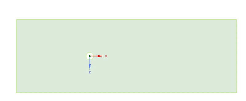
Geometry
- firstly draw a 2m circle.
- draw a 20m line from the center of the circle to the left.
- draw a 10m long line in both upward and downward from the end of the line.
- draw a 40m line from the center of the circle to the right.
- now draw a rectangle from the left corner end to the right line end of dimension 20X40m.
- delete the line 1, 2, 3 and 4.
- now select the inner area of the circle we will get the desired surface.
Meshing
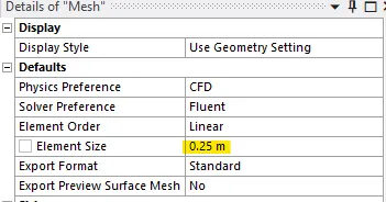
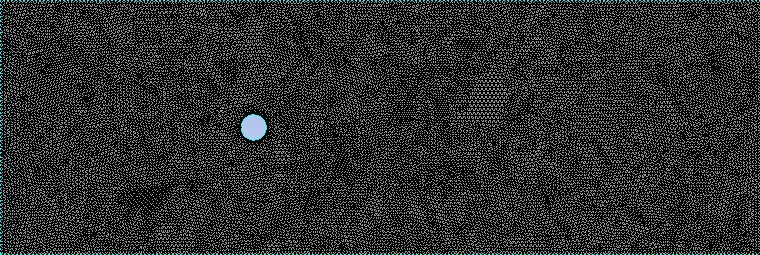
- change the element size from default size to 0.25m.
- insert a mesh method and change the method to triangle.
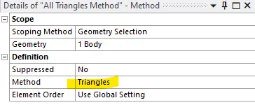
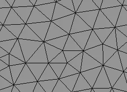
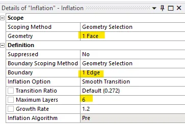
- insert a inflation in mesh and select geometry and apply then select edge and apply.
- now change maximum layers to 6.
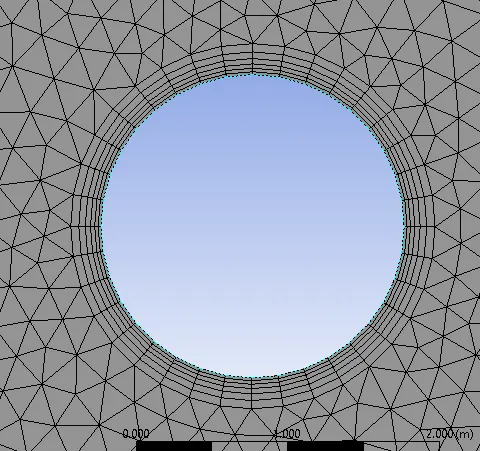
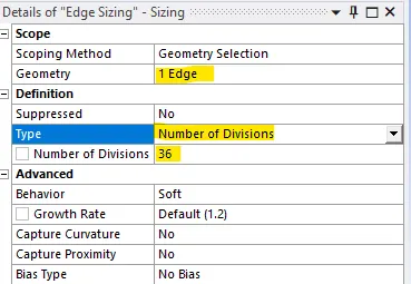
- now insert a sizing method there we will change the edge sizing. since circle is not looking like a circle after zooming in so we will change the edge properties.
- select the geometry and apply now change the type to 'no. of divisions' and change the no. of division to 36.
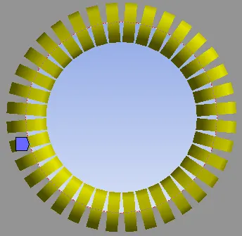
- now generate the mesh and update.
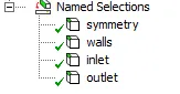
- now assign the names for the boundaries.
Setup
- after opening fluent setup select physics the go to general setting there we will select:
A. pressure based type.
B. absolute velocity formula
C. Steady state solver
D. planer 2D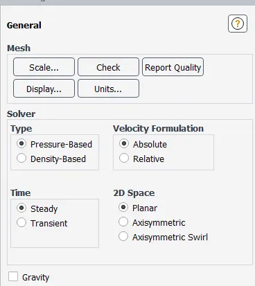
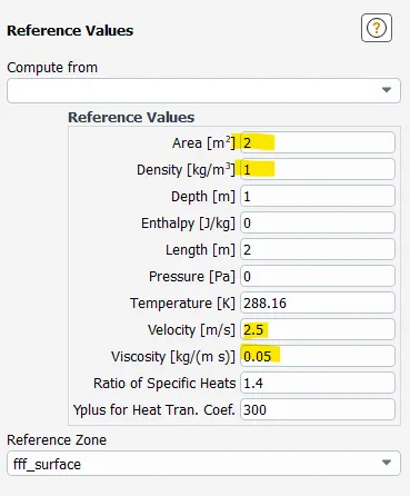
- change reference values as given below:
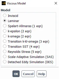
- change the turbulence model to laminar
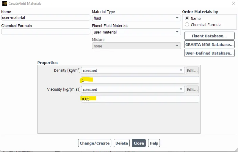
- select an edited user material of density `1Kg/m^3` and viscosity `0.05 Kg/m*s` of type fluid.
- change the boundary conditions.
a. change the inlet velocity as calculated for particular Reynolds number.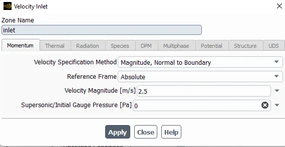
b. for outlet make sure the outlet is pressure outlet and it is set to zero pascal gauge pressure.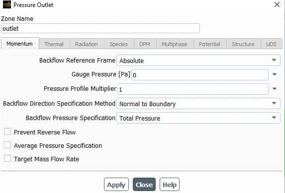
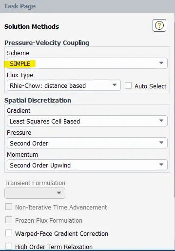
c. make sure that symmetry type is symmetry and cylinder wall type is wall. - now change the solution method pressure velocity coupling to SIMPLE.
- now add report definition for drag and lift coefficient
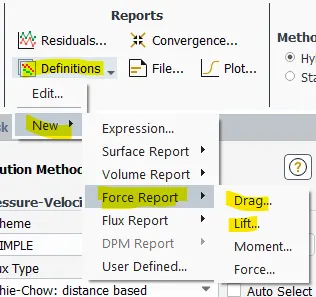
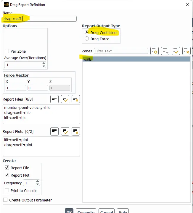
- from results section create a point 'monitor point' 8m away from the center of the circle in x-direction.
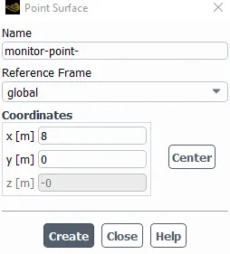
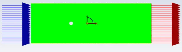
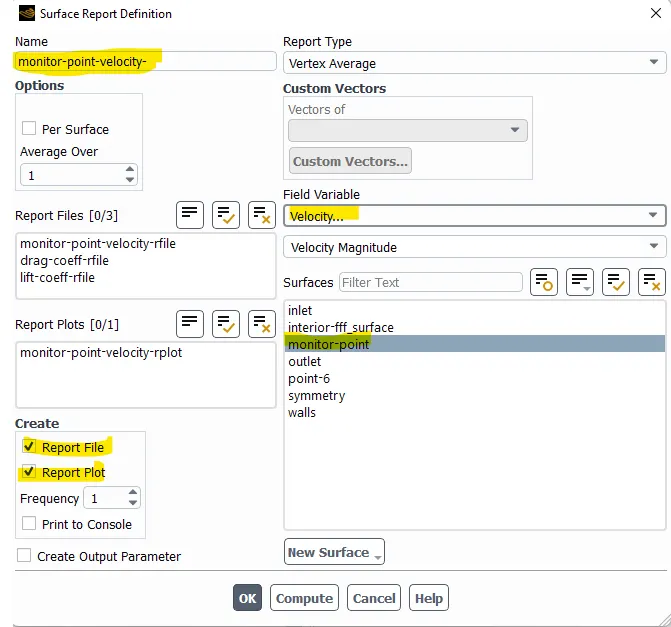
- now create a report definition at monitor point for vertex average velocity.
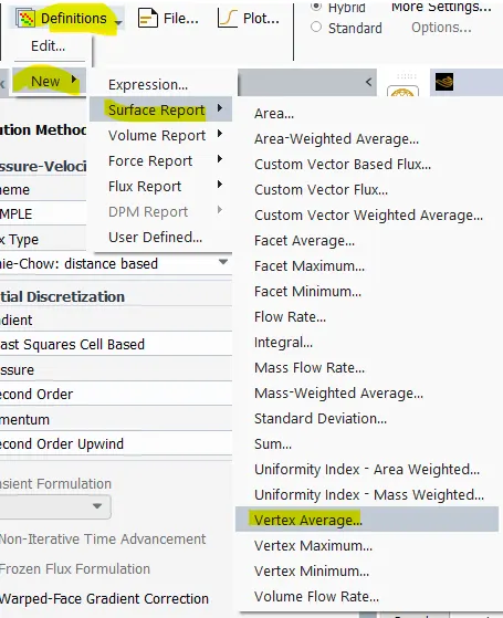
change name => change field variable to velocity=>select monitor point
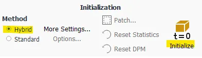
- now initialize the solution with hybrid initialization type.
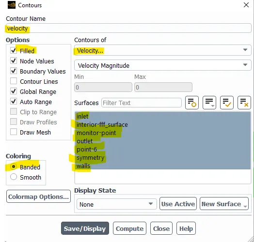
- From results section create pressure and velocity contour.
result=>graphics=>contour=>new - change contour name and variable then select all surfaces
- Open residuals then uncheck convergence so that solution will not stop after converging automatically.
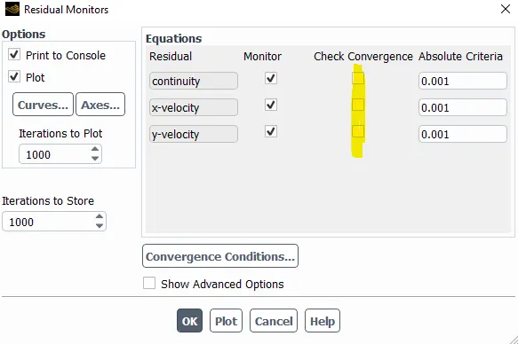
- Now run the simulation
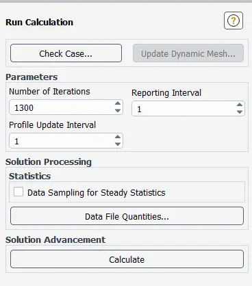
- now add report definition for drag and lift coefficient
Output from the simulation
Velocity contour
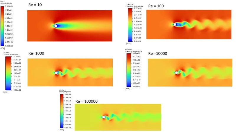
residuals
For Re = 10
For Re = 100
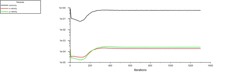
For Re = 1000
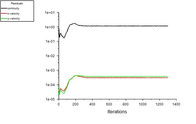
For Re = 10000
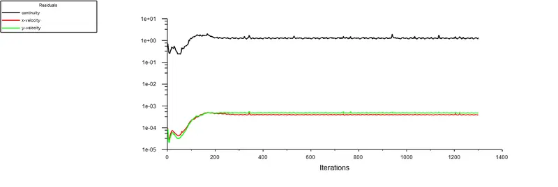
For Re = 100000
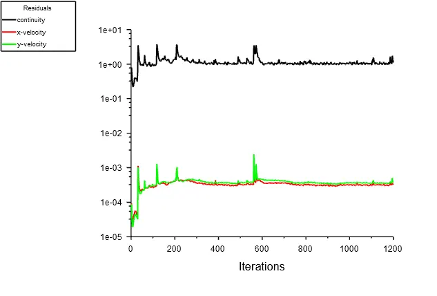
- By looking at residuals plot for lower Reynolds number(10, 100, 1000) we can say that solution has converged, because we can observe that it is almost linear but if we will zoom it actually it is not linear, it is zig zag but it is following a similar pattern so we can say that solution is converged
- but for higher Reynolds number (10000, 100000) it is very difficult to say that solution has converged because we can see the residuals are not following any path. so we can say that solution has not converged for Re = 10000 and 100000.
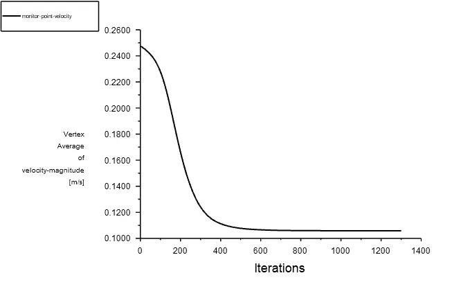
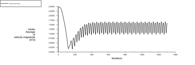
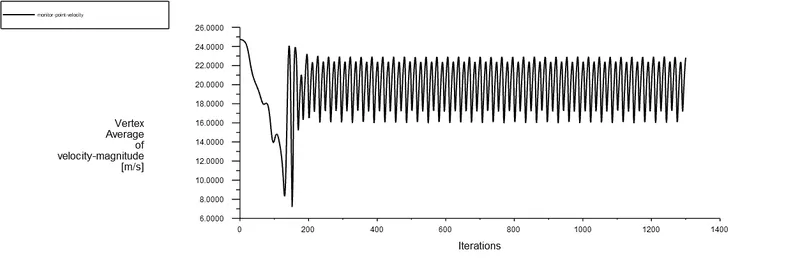
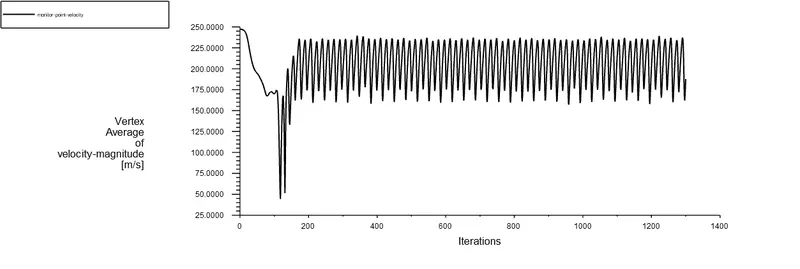
velocity profile at monitor point
For Re = 10
For Re = 100
For Re = 1000
For Re = 10000
For Re = 100000
Coefficient of lift
for Re = 10
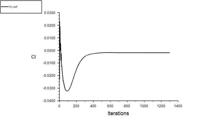
For Re = 100
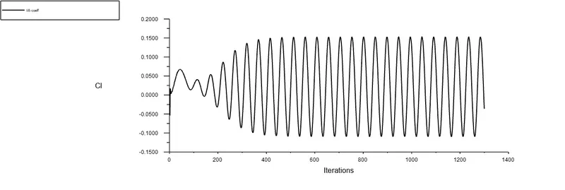
For Re = 1000
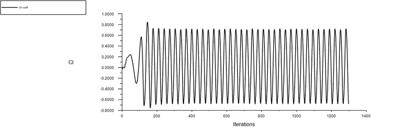
For Re = 10000
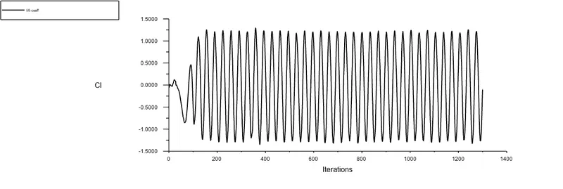
For Re = 100000
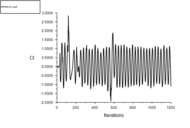
Coefficient of drag
For Re = 10
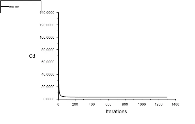
For Re = 100
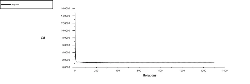
For Re = 1000
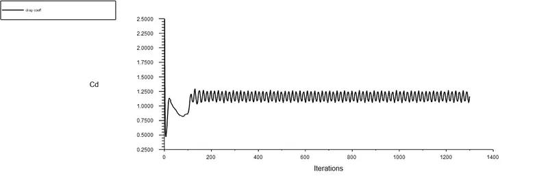
For Re = 10000
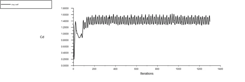
For Re = 100000
- from the above plots of drag coefficient we can observe that as the Reynolds number is increasing the magnitude of drag coefficient is decreasing, as much we are increasing the Reynolds number drag coefficient value is fluctuating. at lower Reynolds number it is linear.
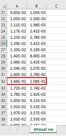
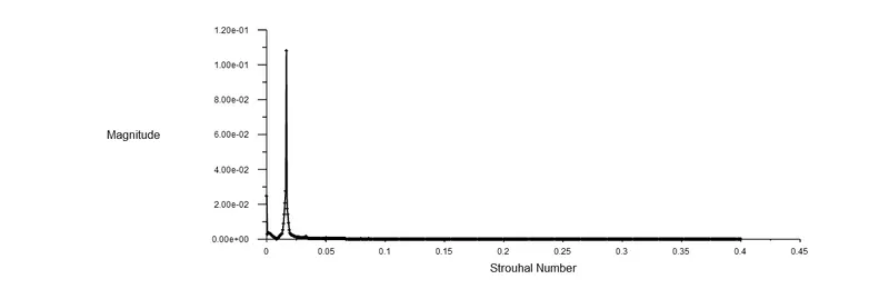
Strouhal number for Re = 100
CASE SETUP FOR TRANSIENT CASE
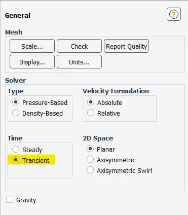
For transient case most of the steps are similar as steady state except
- Transient
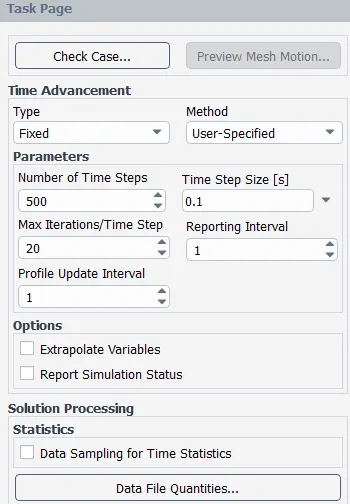
- Solution run method
OUTPUT FOR TRANSIENT STATE SOLUTION
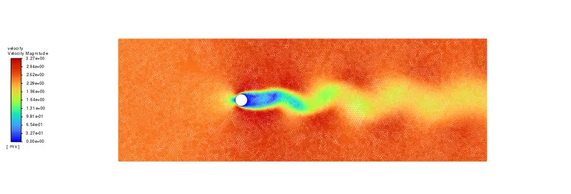
VELOCITY CONTOUR
RESIDUALS
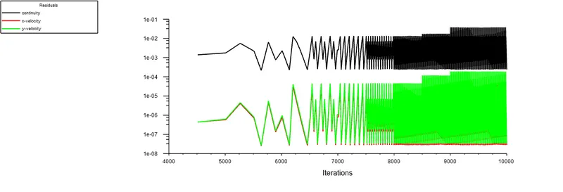
- from the residual plot we can observe that it is following a path like saw tooth, so we can say that solution has converged.
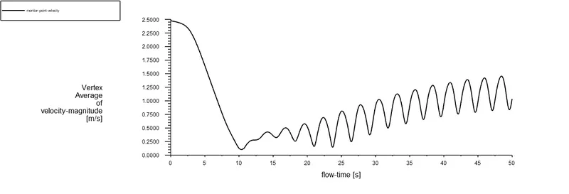
VELOCITY PROFILE AT MONITOR POINT
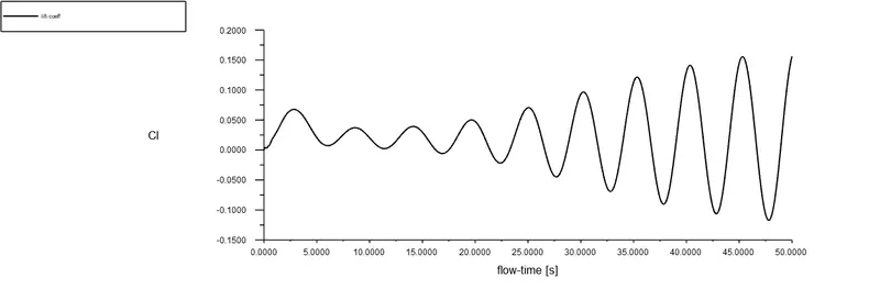
COEFFICIENT OF LIFT
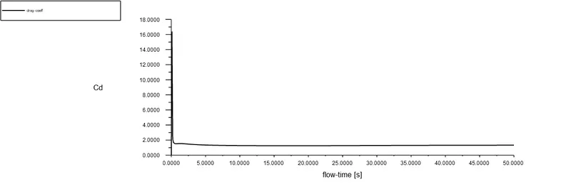
COEFFICIENT OF DRAG
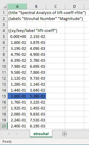
STROUHAL NUMBER
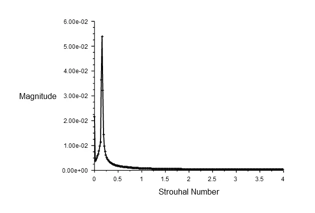
LINK FOR ANIMATION
comparison of drag coefficient with standard data
For Re = 100
standard value = 1.3353
experimental value = 1.3352
`text(% error) = text(experimental data - analytical data)/text(analytical data)xx100`
`text(% error) = (1.3353-1.3352)/1.3353xx100=0.007%`
conclusion
- For lower Reynolds number the vortices does not form, but as we keep n increasing the Reynolds number wakes starts to form, by further increasing the Reynolds number wakes leave the cylinder wall and form vortices. these vertices are symmetrical.
- As we are increasing the Reynolds number vortices height from the center line of the cylinder is increasing.
- Steady state solvers are more faster than the transient state solvers.
Reference
https://www.sciencedirect.com/science/article/pii/S0307904X08000243#tbl2
Fluid Mechanics by Pijush K. Kundu and Ira M. Cohen