Week 2 - Flow over a Cylinder.

Simulate the flow over a cylinder and explain the phenomenon of Karman vortex street.

PART-I

1. Simulate the flow with the steady and unsteady case and calculate the Strouhal Number for Re= 100.

PART-II

1. Calculate the coefficient of drag and lift over a cylinder by setting the Reynolds number to 10,100,1000,10000 & 100000. (Run with steady solver)
   
   
2. Discuss the effect of Reynolds number on the coefficient of drag. [ Results should be validated with any standard literature and error should be within 5 %]

Theory –

Vortex Shedding -

In fluid dynamics, vortex shedding is an oscillating flow that takes place when a fluid such as air or water flows past a bluff (as opposed to a streamlined) body at certain velocities, depending on the size and shape of the body. In this flow, vortices are created at the back of the body and detach periodically from either side of the body forming a Von Karman vortex street which is responsible for the unsteady separation of the flow of a fluid around blunt bodies. It is named after the engineer Theodore Von Karman. The fluid flow past the object creates alternating low-pressure vortices on the downstream side of the object. The object will tend to move toward the low-pressure zone.

A vortex street will form only at a certain range of flow velocities, specified by a range of Reynolds numbers (Re), typically above a limiting Re value of about 90. The Reynolds number for a flow is a measure of the ratio of inertial to viscous forces in the flow of a fluid around a body or in a channel.

`Re = (UL)/v_0`

U = the free stream flow speed

L = a characteristic length parameter of the body or channel

`v_0` = the free stream kinematic viscosity

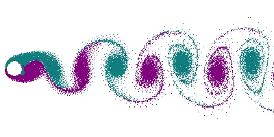
Animation of vortex street created by a cylindrical object; the flow on opposite sides of the object is given different colours, showing that the vortices are shed from alternating sides of the object.

Strouhal Number -

In dimensional analysis, the Strouhal number is a dimensionless number describing oscillating flow mechanisms. For large Strouhal numbers (order of 1), viscosity dominates fluid flow, resulting in a collective oscillating movement of the fluid "plug". For low Strouhal numbers (order of 10-4 and below), the high-speed, quasi-steady-state portion of the movement dominates the oscillation. Oscillation at intermediate Strouhal numbers is characterized by the buildup and rapidly subsequent shedding of vortices.

`S_t = (fD)/(U')`

Where,

f= frequency of vortex shedding

D= characteristic diameter of the cylinder

U'= fluid flow velocity

Co-efficient of drag -

In fluid dynamics, the drag coefficient (`C_d`) is a dimensionless quantity that is used to quantify the drag or resistance of an object in a fluid environment, such as air or water. It is used in the drag equation in which a lower drag coefficient indicates the object will have a less aerodynamic or hydrodynamic drag. The drag coefficient is always associated with a particular surface area.

The drag coefficient of any object comprises the effects of the two basic contributors to fluid dynamic drag: skin friction and form drag. The drag coefficient of a lifting airfoil or hydrofoil also includes the effects of lift-induced drag. The drag coefficient of a complete structure such as an aircraft also includes the effects of interference drag.

The drag coefficient (`C_d`)is defined as

`C_d = (2.F_d)/(ρu^2 A)`

where:

`F_d` is the drag force, which is by definition the force component in the direction of the flow velocity.

`ρ` is the mass density of the fluid,

u is the flow speed of the object relative to the fluid,

A is the reference area.

Co-efficient of lift -

The lift coefficient (`C_L`) is a dimensionless coefficient that relates the lift generated by a lifting body to the fluid density around the body, the fluid velocity, and an associated reference area. A lifting body is a foil or a complete foil-bearing body such as a fixed-wing aircraft. `C_L` is a function of the angle of the body to the flow, its Reynolds number, and its Mach number. The section lift coefficient refers to the dynamic lift characteristics of a two-dimensional foil section, with the reference area replaced by the foil chord.

`C_L = (L)/(qS)=(L)/(1/2ρu^2S)=(2L)/(ρu^2S)`

where

L is the lift force,

S is the relevant surface area and

q is the fluid dynamic pressure, in turn, linked to the fluid density, and to the flow speed.

PROCEDURE -

1.) Geometry -

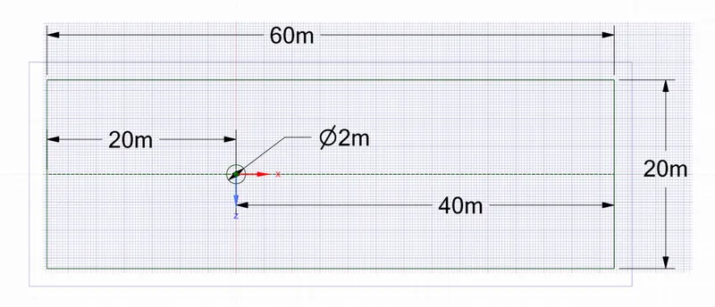
A cylindrical boundary with the required domain for simulation has to be made in SpaceClaim as shown below.

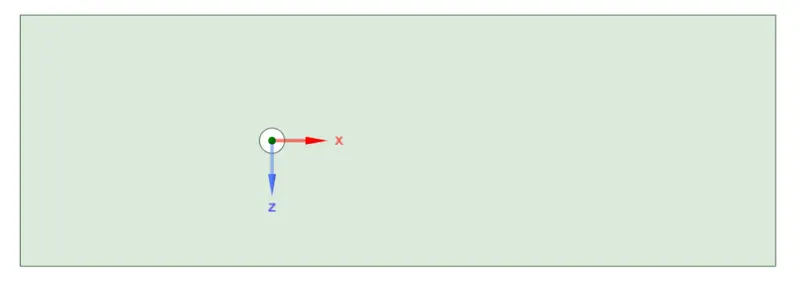
After making the geometry we have to make it a surface with the cylinder part cut out. The final model is shown below.

2.) Mesh -

After the geometry completion, we move to create our mesh for the said geometry.

During the meshing phase-only we have to create out named selection in order to let Ansys know where the inlet, outlet and etc are present as shown below.

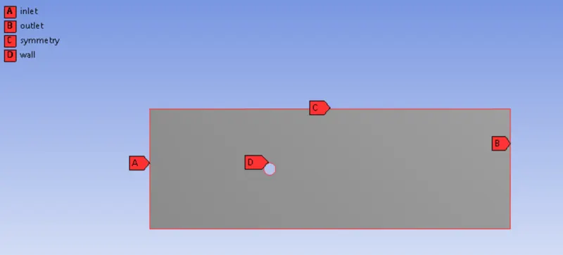
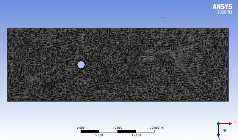
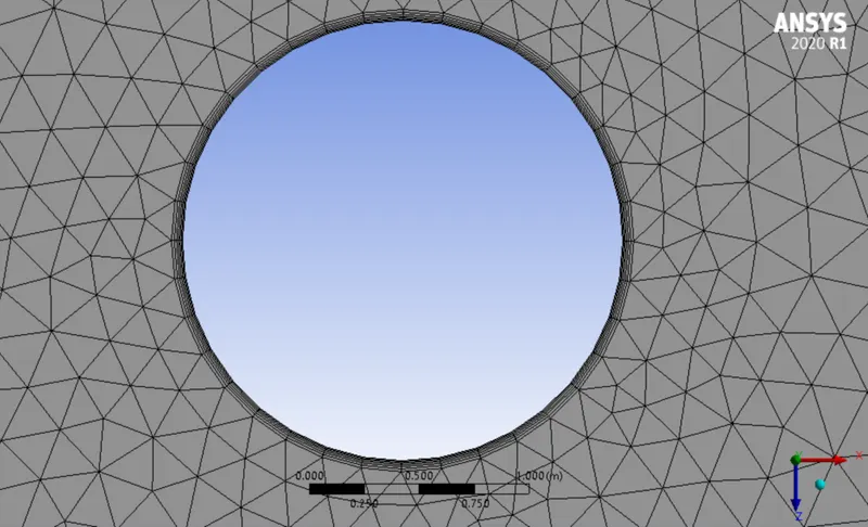
Mesh with element size = 0.25m and inflation layers (6 layers) near the cylinder in order to capture the details more accurately near it is used as shown below.

In order to see if the mesh we have generated is accurate or not, we'll check a quantity known as orthogonal mesh quality which tells us about the quality of our mesh.

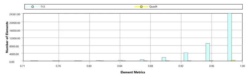
number of elements - 40,502

3.) Solver -

The first thing that we do is to select which type of solver we want to use that is either a steady-state solver or a transient state solver. We'll also have to give reference values for the calculation of drag and lift and we'll have to choose the laminar flow method only. All of which are shown below.

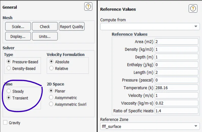
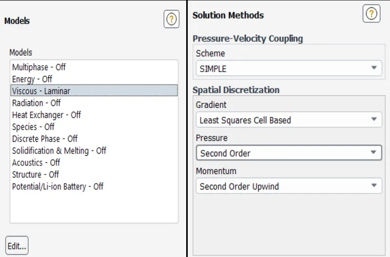
Here, Area = Height*Width = 2m²

Height = 2m

Width = 1m because analysis is 2D

For all 2D problems Depth =1m

Length = 2m (because here length means flow length along the direction of flow which is the diameter = 2m)

Since we need a laminar flow, we'll have to keep the Reynolds number low and in order to do that we'll have to create a user-defined fluid that will have user-defined density and viscosity as shown below.

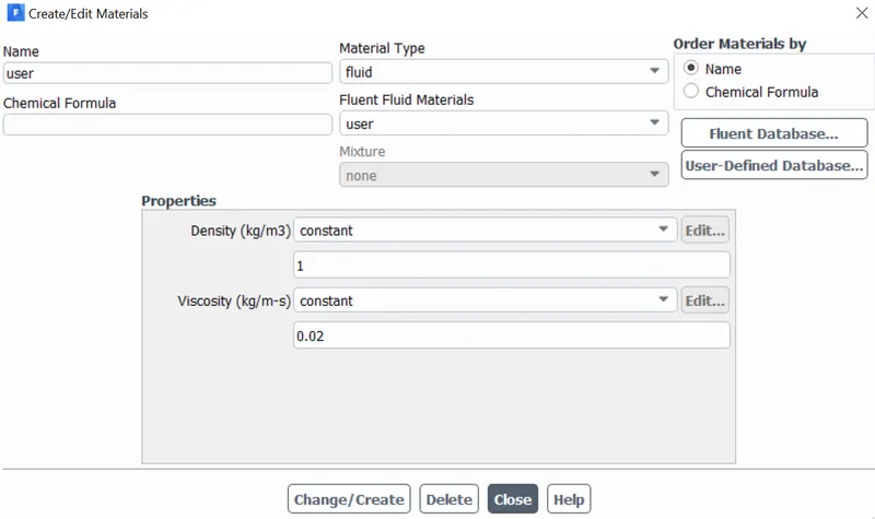
Now as we're done with setting up the solver, we can proceed to run the solver to get the desired result.

Plots –

In both i.e., steady and unsteady state simulations, the following plots are to be shown:

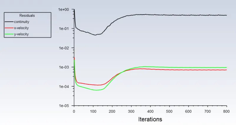
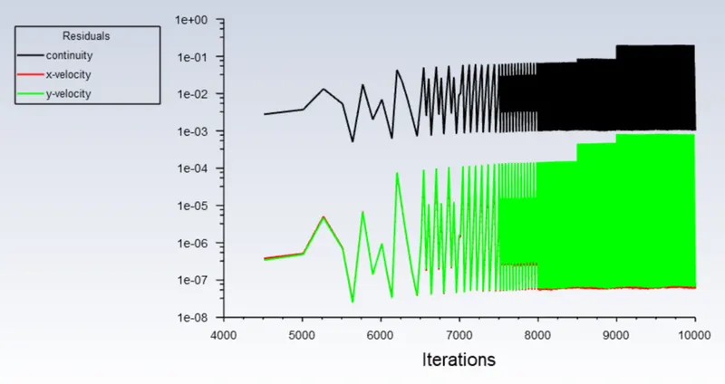
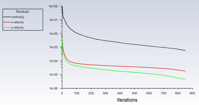
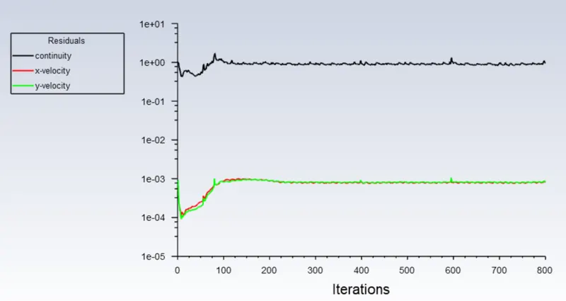
1. Residual plot - This plot helps us in knowing at what point convergence is achieved.
   
   
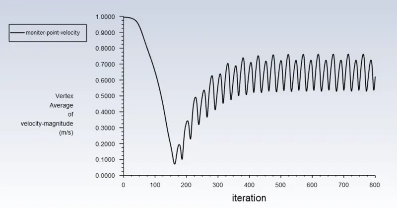
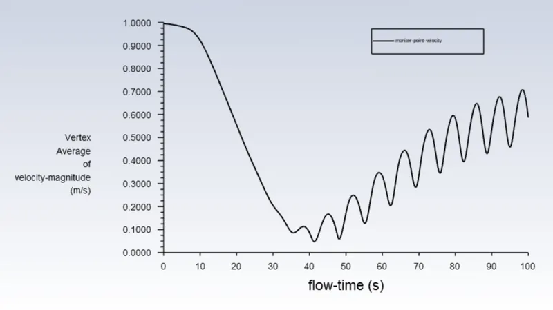
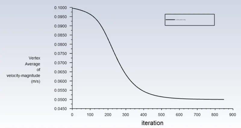
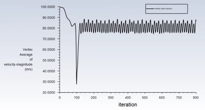
2. Monitor point velocity plot - A monitor point is placed at a distance of 8m from the cylinder in order to calculate the velocity at that point.
   
   
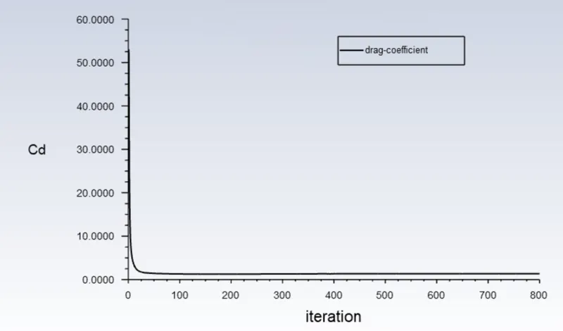
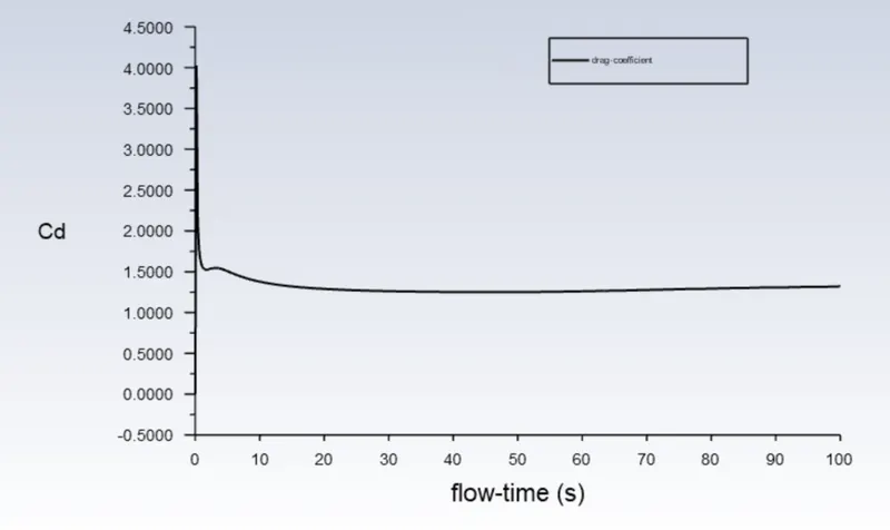
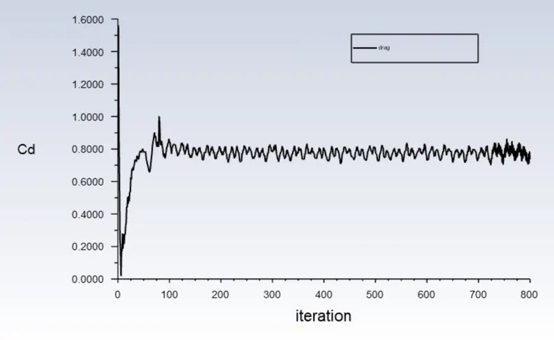
3. Drag coefficient plot - To calculate the drag coefficient.
   
   
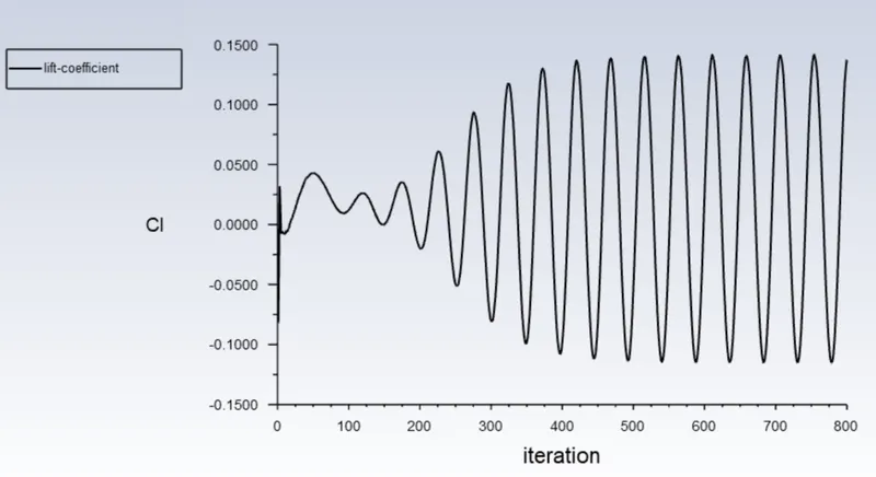
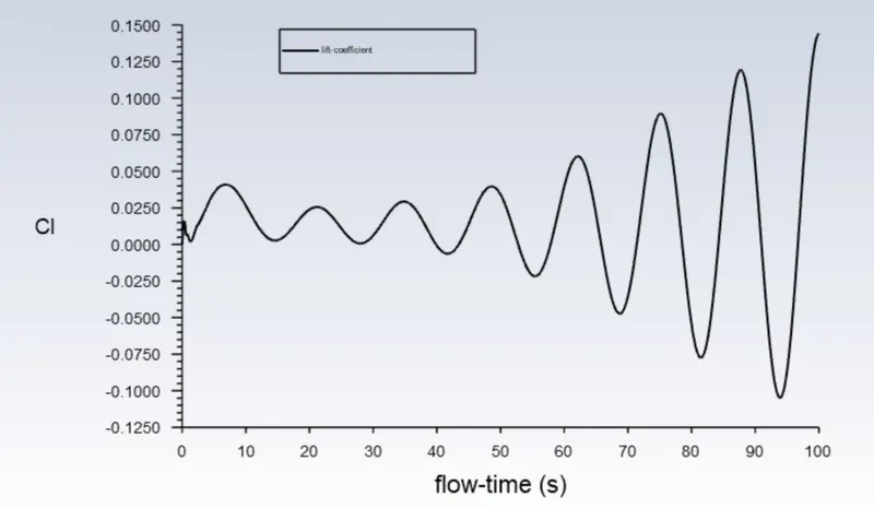
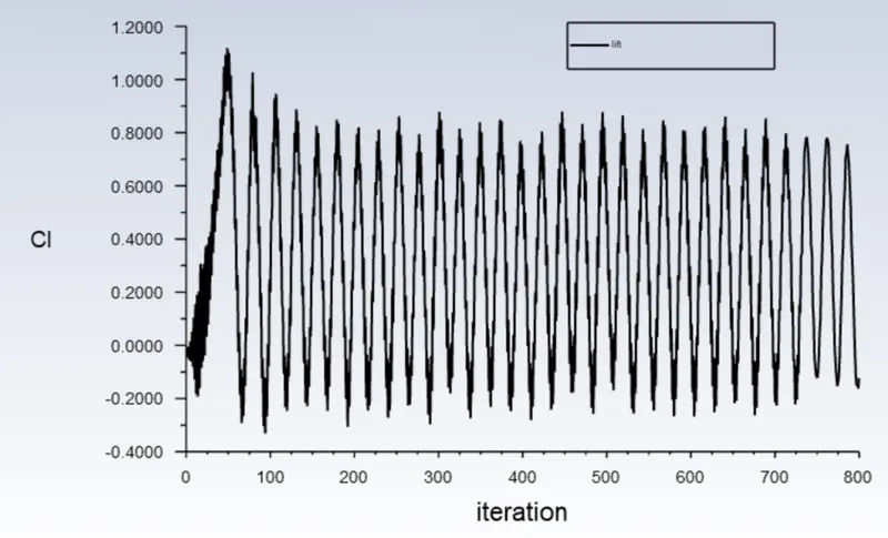
4. Lift coefficient plot - To calculate the lift coefficient.
   
   
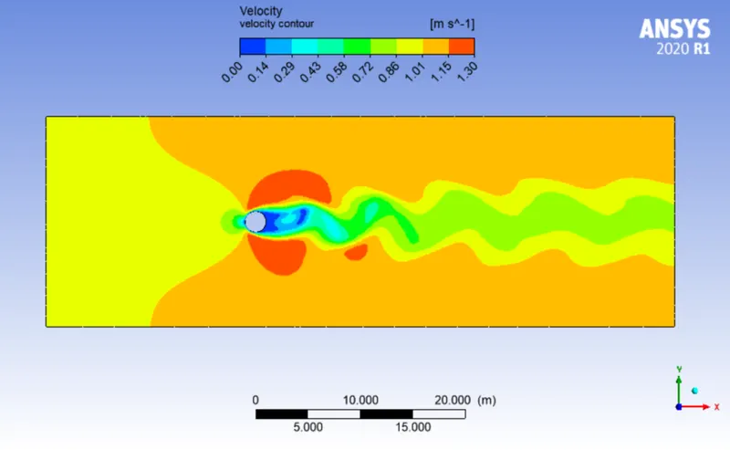
5. Velocity contour - To see the velocity changes in the flow over the cylinder.
   
   
6. Pressure contour - To see the Pressure changes in the flow over the cylinder.

PART 1 -

STEADY-STATE SIMULATION -

For Re = 100 where viscosity = 0.02 and velocity = 1m/s

Residual Plot -

Monitor Point Velocity -

Drag Coefficient -

Lift Coefficient -

Velocity Contour -

Strouhal Number Plot -

We can use the FFT option to get the strouhal number plot and then write that data into excel in order to get the maximum magnitude and hence the corresponding strouhal number.

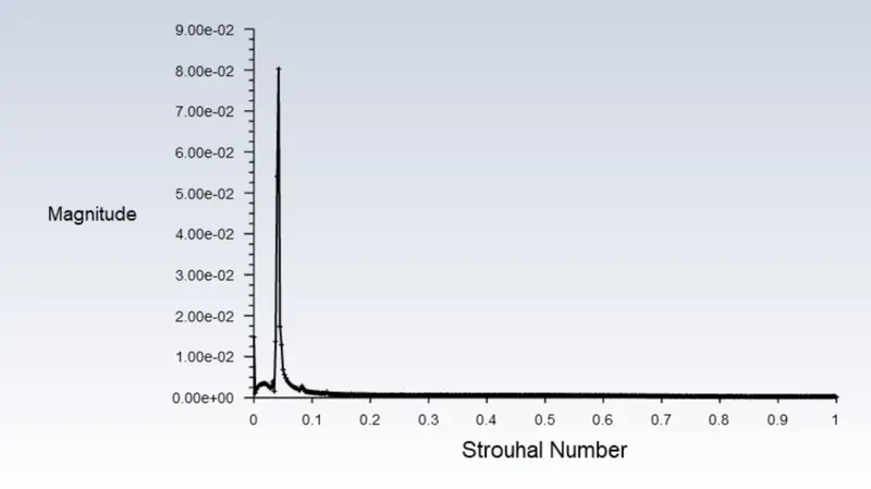
Strouhal number = 0.0425 for steady state case.

TRANSIENT-STATE SIMULATION -

For Re = 100 where viscosity = 0.02 ,velocity = 1m/s ,Time interval = 0.2 and iterations = 500

Residual Plot -

Monitor Point Velocity -

Drag Coefficient -

Lift Coefficient -

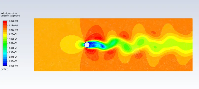
Velocity Contour -

Strouhal Number Plot -

We can use the FFT option to get the strouhal number plot and then write that data into excel in order to get the maximum magnitude and hence the corresponding strouhal number.

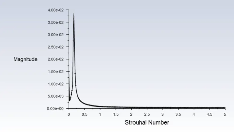
Strouhal number = 0.15968 for transient state case.

PART 2 -

STEADY-STATE SIMULATION -

1.) Case 1 -

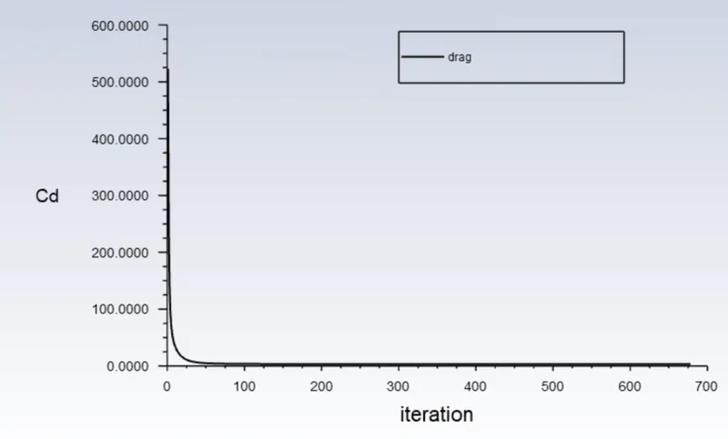
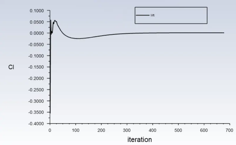
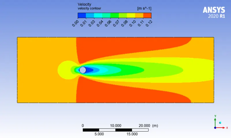
For Re = 10 where viscosity = 0.02 and velocity=0.1m/s

Residual Plot -

Monitor Point Velocity -

Drag Coefficient -

Lift Coefficient -

Velocity Contour -

2.) Case 2 -

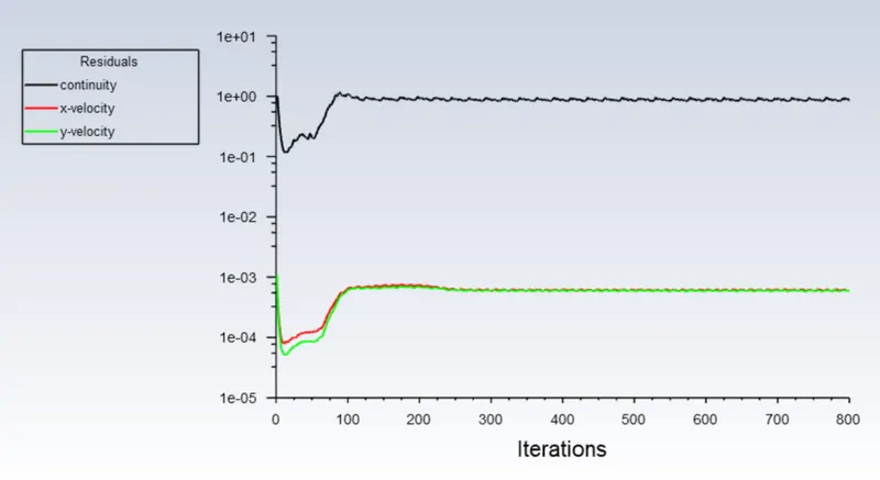
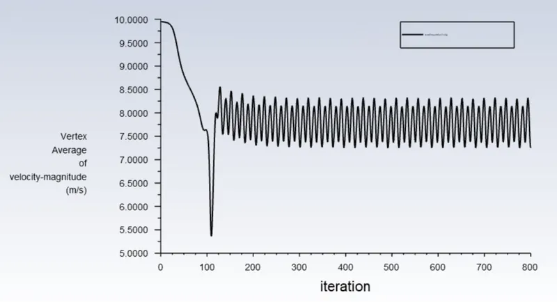
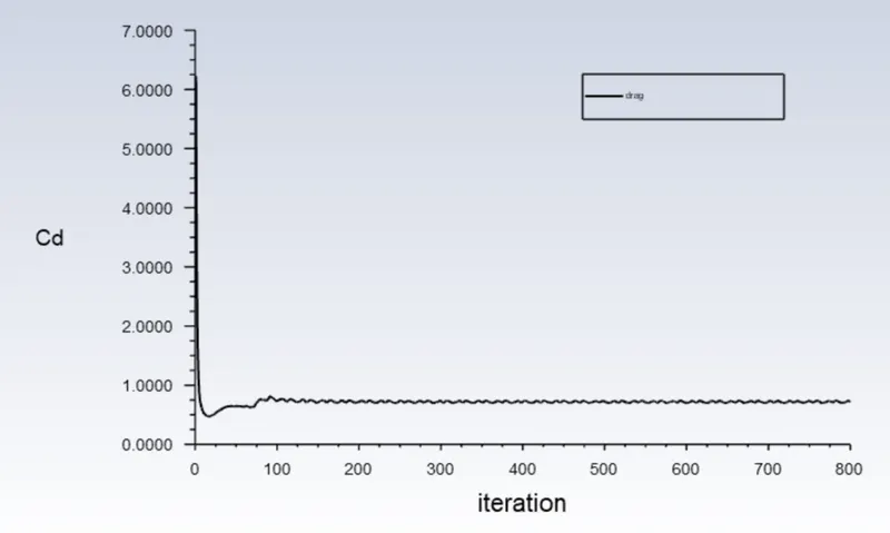
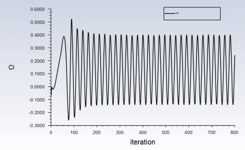
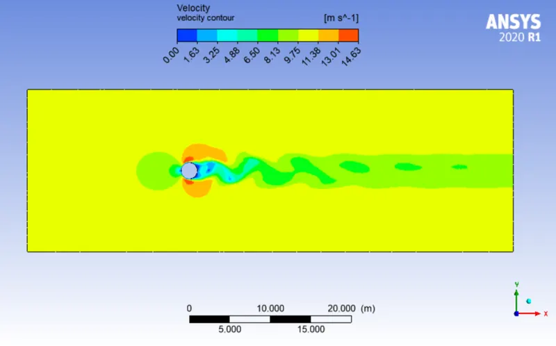
For Re = 1,000 where viscosity = 0.02 and velocity = 10m/s

Residual Plot -

Monitor Point Velocity -

Drag Coefficient -

Lift Coefficient -

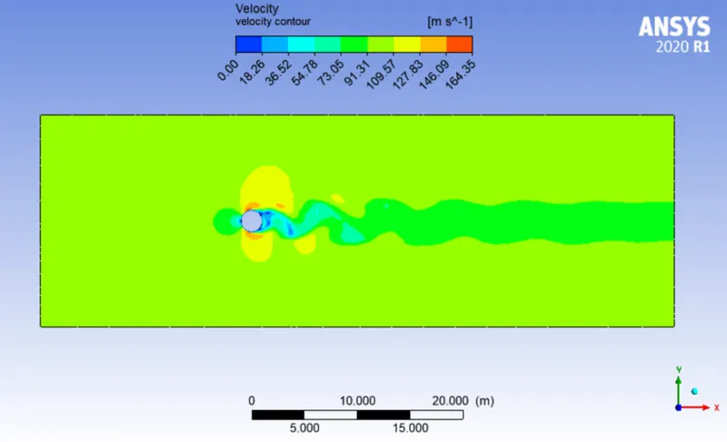
Velocity Contour -

3.) Case 3 -

For Re = 10,000 where viscosity = 0.02 and velocity = 100m/s

Residual Plot -

Monitor Point Velocity -

Drag Coefficient -

Lift Coefficient -

Velocity Contour -

4.) Case 4 -

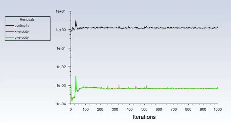
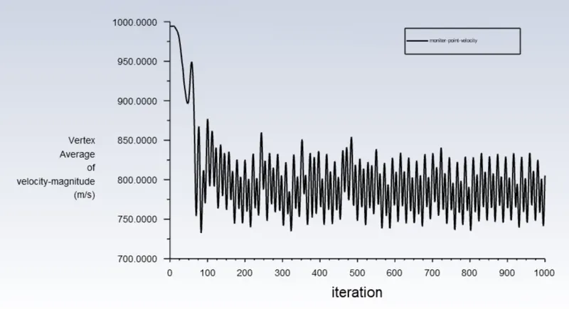
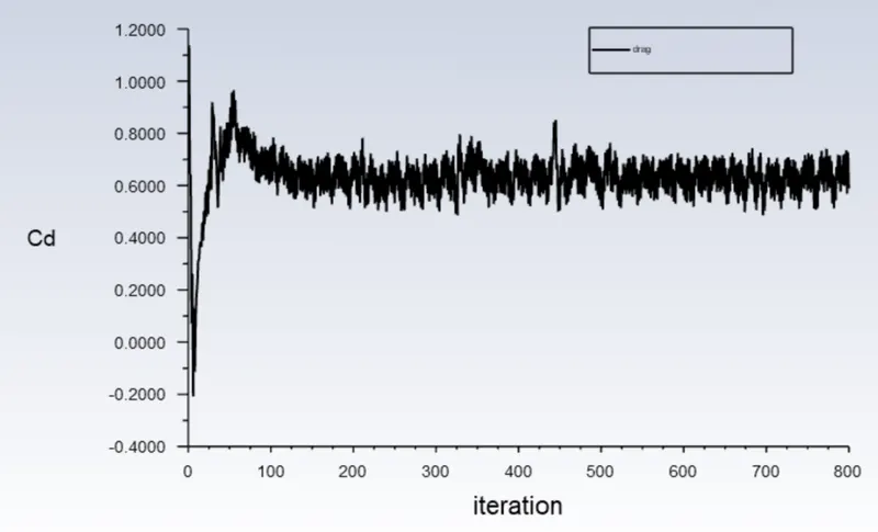
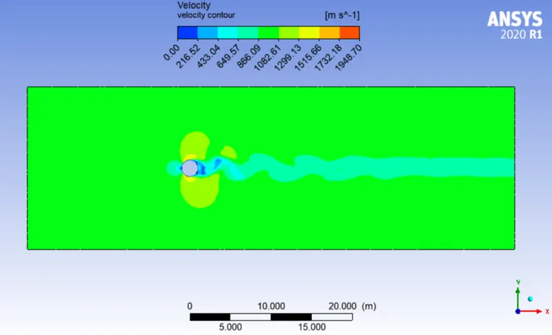
For Re = 1,00,000 where viscosity = 0.02 and velocity = 1,000m/s

Residual Plot -

Monitor Point Velocity -

Drag Coefficient -

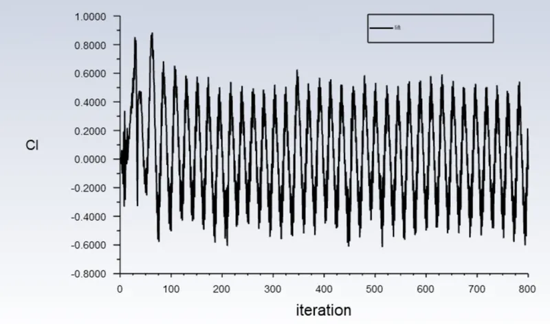
Lift Coefficient -

Velocity Contour -

RESULT -

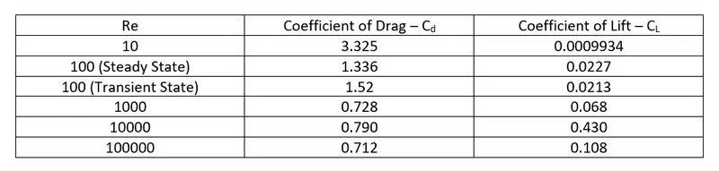
Drag and lift coefficient for different Re.

Conclusion -

• In the first case, the flow over a cylinder is simulated for both Steady and unsteady cases with Re=100, and with the results generated the phenomena of Von Karman Vortex Street are also observed.
  
  
• Necessary plots are plotted in order to observe that the flow is converged and the vortex shedding is happening.
  
  
• Contours are generated in order to observe the flow over a cylinder.
  
  
• By plotting the Magnitude vs Strouhal number, the Strouhal number is calculated by seeing the maximum magnitude using the data in excel.
  
  
• The transient model is appropriate for the Vortex Karman Street phenomenon as it is time-dependent.

In the second case,

• Six different simulations i.e. (Re = 10,100,1000,10000,100000,1000000) are simulated to observe the behaviour of the drag and lift coefficients by changing the inlet velocity.

• The increase in Re leads to the shedding of vortices from upper- and lower-cylinder surfaces at a particular frequency. At lower Re=10, there is no formation of vortices. Vortex shedding takes place at higher Re like 100, 1000, 10000 and 100000 from the above results obtained from simulation.

• As Re is increased it can be seen that the coefficient of drag decreases.
• As per the basic conditions and parameters, the results are validated from the literature.
  
  
• As we refine the mesh, we need to run more iterations.
  
  
• From the above table, it can be concluded that the error percentage is less than 5%.

References -

[1] Numerical simulation of laminar flow past a circular cylinder, CTFD Division, National Aerospace Laboratories, Airport Road, Bangalore.