Explicit and Implicit Analysis
Aim:
To solve the equation `u^3+9u^2+4u` using Explicit and Implicit Methods.
Explicit and implicit Analysis:
Explicit and implicit methods are approaches used in numerical analysis for obtaining numerical approximations to the solutions of time-dependent ordinary and partial differential equations, as is required in computer simulations of physical processes. Explicit methods calculate the state of a system at a later time from the state of the system at the current time, while implicit methods find a solution by solving an equation involving both the current state of the system and the later one. Mathematically, if Y(t) is the current system state and Y(t +`Delta t`) is the state at the later time (`Deltat` is a small time step), then, for an explicit method.
Explicit Method:
Force, `F(u) = u^3 + 9u^2 + 4u`
Stiffness , `k(u) = d/(du)F(u) = 3u^2 + 18u + 4`
Displacement = Force/Stiffness = `F/k`
Force increment = dF = 1
Displacement increment, `du = (dF)/k`
Displacement, `u_(i+1) = u_i + du_i`
Step 1:
dF = 1
`k(u_0) = 3(u_0)^2 + 18u_0 + 4`
`k(u_0) = 3(0)^2 + 18(0) + 4`
`k(u_0) = 4`
`du_1 = (dF)/(k(u_0)) = 1/4 = 0.25`
`u_1 = u_0 + du_1 = 0 + 0.25 = 0.25`
`F(u_1) = (u_1)^3 + 9(u_1)^2 + 4u_1`
`F(u_1) = (0.25)^3 + 9(0.25)^2 + 4(0.25)`
`F(u_1) = 1.578`
`F_(ext) = dF = 1`
`u_(exact) = 0.177`
by solving the cubic polynomial `F_(ext) = (u_(ext))^3 + 9(u_(ext))^2 + 4(u_(ext))` where `F_(ext) = 1`
Step 2:
dF = 1
`k(u_1) = 3(u_1)^2 + 18(u_1) + 4`
`k(u_1) = 3(0.25)^2 + 18(0.25) + 4`
`k(u_1) = 8.688`
`du_2 = (dF)/(k(u_1)) = 1/8.688 = 0.115`
`u_2 = u_1 + du_2 = 0.25 + 0.115 = 0.365`
`F(u_2) = (u_2)^3 + 9(u_2)^2 + 4(u_2)`
`F(u_2) = (0.365)^3 + 9(0.365)^2 + 4(0.365)`
`F(u_2) = 2.709`
`F_(ext) = dF + dF = 1 +1 = 2`
`u_(exact) = 0.296`
`y solving the cubic polynomial `F_(ext) = (u_(exact))^3 + 9(u_(exact))^2 + 4(u_(exact))` where `F_(exact) = 1`
Step 3:
dF = 1
`k(u_2) = 3(u_2)^2 + 18(u_2) + 4`
`k(u_2) = 3(0.365)^2 + 18(0.365) + 4`
`k(u_2) = 10.972`
`du_3 = (dF)/(k(u_2)) = 1/10.972 = 0.091`
`u_3 = u_2 + du_3 = 0.365 + 0.091 = 0.456`
`F(u_3) = (u_3)^3 + 9(u_3)^2 + 4(u_3)`
`F(u_3) = (0.456)^3 + 9(0.456)^2 + 4(0.456)`
`F(u_3) = 3.793`
`F_(ext) = dF + dF + dF = 1 + 1 + 1 = 3`
`u_(exact) = 0.391`
by solving the cubic polynomial `F_(exact) = (u_(exact))^3 + 9(u_(exact))^2 + 4(u_(exact))` where `F_(exact) = 3`
| Step | `u_i` | `dF` | `k(u_i)` | `du_i = (dF)/(k(u_i))` | `u_(i+1)` | `F_(ext)` | `F_(Int)` | `R = F_(Int) - F_(ext)` | `U_(exact)` |
| 0 | 0 | 0 | 4 | 0 | 0.25 | 0 | 0 | 0 | 0 |
| 1 | 0.25 | 1 | 8.688 | 0.25 | 0.365 | 1 | 1.578 | 0.578 | 0.177 |
| 2 | 0.365 | 1 | 10.972 | 0.115 | 0.456 | 2 | 2.709 | 0.709 | 0.296 |
| 3 | 0.456 | 1 | 12.837 | 0.091 | 0.534 | 3 | 3.793 | 0.793 | 0.392 |
Implicit Method:
In Implicit method at the end of each step Newton-Raphson iterations are used to enforce equilibrium before moving to the next step. internal forces and external forces will not be in equilibrium unless the stiffness is linear for the given step. Hence, in order to achieve equilibrium, corrections must be made to the displacement.
This is accomplished by using Newton-Raphson iterations to minimize the residual, `R(u) = f_(Int) - F_(ext)`
Expanding the residual as a Taylor series about the current displacement `u^j` gives
`R^(j+1) = R^j (u^j) + (dR(u^j))/(du) delu^(j+1) + ... = R^j + k(u^j) delu^(j+1) + ...`
By neglecting higher order terms in the series, setting `R^(j+1) = 0` and solving for `delu^(j+1)` the following correction is obtained
`delu^(j+1) = - [k(u^j)]^-1 R^j`
Force Function, `F(u) = u^3 + 9u^2 + 4u`
Stiffness, `k(u) = d/(du)F(u) = 3u^2 + 18u + 4`
Displacement = Force/Stifness = `F/k`
Force increment = dF = 1
Displacement increment, `du = (dF)/k`
Displacement, `u_(i+1) = u_i + du_i`
Step 1:
`dF =1`
`k(u_0) = 3(u_0)^2 + 18(u_0) + 4`
`k(u_0) = 3(0)^2 + 18(0) + 4 = 4`
`du_1 = (dF)/(k(u_0)) = 1/4 = 0.25`
`u_1 = u_0 + du_1 = 0 + 0.25 = 0.25`
`F(u_1) = (u_1)^3 + 9(u_1)^2 + 4(u_1)`
`F(u_1) = (0.25)^3 + 9(0.25)^2 + 4(0.25) = 1.578`
`F_(ext) = dF = 1`
`R = F(u_1) - F_(ext) = 1.578 -1 = 0.578`
since `||R|| > 0.01` Newton-Raphson iterations have to be done to obtain a correction factor to bring the R value within the tolerance.
i.
`u_1^0 = u_1 = 0.25`
correction factor for `u_1 = delu_1^((1)) = -[k(u_1^((0)))]^-1R^0`
`k(u_1^((0))) = k(u_1) = 3(0.25)^2 + 18(0.25) + 4 = 8.688`
`R^((0)) = 0.578`
`delu_1^((1)) = -[8.688]^-1 * 0.578 = -0.00665`
Corrected `u_1 = u_1^((1)) = u_1 + delu_1^((1)) = 0.25 + (-0.00665) = 0.183`
`F^((1)) = ((u_1^((1)))^3 + 9(u_1^((1)))^2 + 4(u_1^((1)))`
`F^((1)) = (0.183)^3 + 9(0.183)^2 + 4(0.183) = 1.039`
Residual, `R^((1)) = F^((1)) - F_(ext) = 1.039 - 1 = 0.039`
`||R||` is not within tolerance limit.
ii. correction factor for `u_1 = delu_1^((2)) = delu_1^((1)) - [k(u_1^((1)))]^-1 R^((1))`
`k(u_1^((1))) = 3(0.183)^2 + 18(0.183) + 4 = 7.394`
`R^((1)) = 0.039`
`delu_1^((2)) = -0.0665 - [7.394]^-1 * 0.039 = -0.0718`
Corrected `u_1^((2)) = u_1 + delu_1^((2)) = 0.25 + (-0.0718) = 0.1782`
`F^((2)) = (0.1782)^3 + 9(0.1782)^2 + 4(0.1782) = 1.004`
Residual, `R^((2)) = F^((2)) - F_(ext) = 1.004 - 1 = 0.004`
`||R|| < 0.01` within tolerance limit.
Step 2:
dF = 1
`k(u_1) = 3(u_1)^2 + 18(u_1) + 4`
`k(u_1) = 3(0.1782)^2 + 18(0.1782) + 4 = 7.302`
`du_2 = (dF)/(k(u_1)) = 1/7.302 = 0.137`
`u_2 = u_1 + du_2 = 0.1782 + 0.137 = 0.315`
`F(u_2) = (0.315)^3 + 9(0.315)^2 + 4(0.315) = 2.184`
`F_(ext) = dF + dF = 1 + 1 = 2`
`R = F(u_2) - F_(ext) = 2.184 - 2 = 0.184`
`||R|| > 0.01`
Iteration
`u_2^((0)) = u_2`
`k(u_2^((0))) = k(u_2) = 9.967`
`R^((0)) = 0.184`
Correction Factor for `u_2 = delu_2^((1)) = -[k(u_2^((0)))]^-1R^((0))`
`delu_2^((1)) = -[9.967]^-1* 0.184 = -0.0185`
Corrected `u_2 = u_2^((1)) = u_2 + delu_2^((1)) = 0.315 + (-0.0185) = 0.296`
`F^((1)) = (0.296)^3 + 9(0.296)^2 + 4(0.296) = 1.998`
Residual `R^((1)) = F^((1)) - F_(ext) = 1.998 - 2 = -0.002`
`||R|| < 0.01` within the tolerance limit
Step 3:
dF = 1
`k(u_2) = 3(0.296)^2 + 18(0.296) + 4 = 9.59`
`du_3 = 1/9.59 = 0.104`
`u_3 = u_2 + du_3 = 0.296 + 0.104 = 0.4`
`F(u_3) = (0.4)^3 + 9(0.4)^2 + 4(0.4) = 3.104`
`F_(ext) = dF + dF + dF = 1 + 1 + 1 = 3`
`R = F(u_3) - F_(ext) = 3.104 - 3 = 0.104`
`||R|| > 0.01`
Iteration
`u_3^((0)) = u_3 = 0.4`
`k(u_3^((0))) = k(u_3) = 3(0.4)^2 + 18(0.4) + 4 = 11.68`
`R^((0)) = 0.104`
Correction Factor for `u_3 = delu_3^((1)) = -[k(u_3^((0)))]^-1R^((0))`
`delu_3^((1)) = -[11.68]^-1* 0.104 = -0.0089`
Corrected `u_3 = u_3^((1)) = u_3 + delu_3^((1)) = 0.4 + (-0.0089) = 0.3911`
`F^((1)) = (0.3911)^3 + 9(0.3911)^2 + 4(0.3911) = 3.0008`
Residual, `R^((1)) = F^((1)) - F_(ext) = 3.0008 - 3 = 0.0008`
`||R|| < 0.01`
| Step i | `u_i` | Corrected `u_i` | `dF` | `F_(ext)` | `F_(Int)` | Corrected`F_(Int)` | `R = F_(Int) - F_(ext)` | Corrected R | `u_(exact)` |
| 0 | 0 | 0 | 0 | 0 | 0 | 0 | 0 | 0 | 0 |
| 1 | 0.250 | 0.178 | 1 | 1 | 1.5781 | 1.0043 | 0.578 | 0.0043 | 0.177 |
| 2 | 0.365 | 0.296 | 1 | 2 | 2.7088 | 1.9985 | 0.709 | -0.0015 | 0.296 |
| 3 | 0.456 | 0.391 | 1 | 3 | 3.7935 | 3.0009 | 0.793 | 0.0009 | 0.391 |
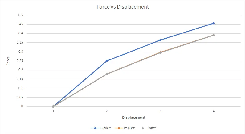
| Step i | Force | Explicit | Implicit | Exact |
| 0 | 0 | 0 | 0 | 0 |
| 1 | 1 | 0.25 | 0.178 | 0.177 |
| 2 | 2 | 0.365 | 0.297 | 0.296 |
| 3 | 3 | 0.456 | 0.391 | 0.391 |
Plot:
Result:
From the above plot the implicit and exact values are same and the explicit values diverge away from the exact values since there is no equilibrium between the internal and external forces. Thus implicit method is prefered for analysis.