Week - 2 - Explicit and Implicit Analysis
Week - 1 - Explicit and Implicit Analysis
Question
Referring to the attached PDF, solve the following equation using implicit and explicit methods with a tolerance of 0.001.
`f(u) = u^3+9u^2+4u`
Answers
Structural Analysis
Structural analysis is the process of predicting how a structure responds to various forces and loads. It involves calculating the effects of these loads on a structure, building or object to ensure that it can safely withstand them. This analysis is vital during the design, testing, or post-construction phases to ensure that the structure can withstand the anticipated loads without failing.
In engineering, structural analysis is crucial for determining a structure's internal forces, stresses, and displacements. It ensures that the structure complies with safety and serviceability criteria as per the relevant codes and standards.
In FEA, it involves breaking down a complex structure into smaller, manageable finite elements that can be analysed more easily. This process helps to understand the behaviour of structures under different loading conditions and is essential for ensuring safety and reliability.
A brief overview of structural analysis in FEA is given below.
- Meshing:
Dividing a structure into a finite number of elements (Discretizing). The quality of the mesh is vital for the accuracy of analysis. - Material Properties:
Assigning accurate material properties is essential as they define how the structure will behave under the load. - Boundary Conditions:
The constraints applied to the model to simulate real-world conditions. - Solving:
The FEA software computes the equations that describe the behaviour of each element. - Post-Processing:
After solving, results are interpreted to make engineering decisions.
This can be used for linear, nonlinear, static, dynamic and thermal analyses, among others.
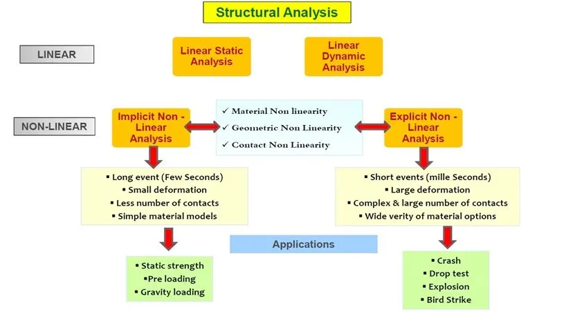
Explicit Analysis
Explicit analysis is a type of dynamic analysis used in FEA. It is particularly effective for solving problems where physical events occur over a very short time, such as impacts, explosions and high-speed dynamic events. The explicit method is capable of handling large deformations and complex contact interactions with greater efficiency in these cases, compared to the implicit method which might be computationally intensive for such analyses.
- Directly calculates the model's state at a new time based on its current state.
- Typically used for problems with dynamic effects where the time steps are very less.
- It does not require matrix inversion. making it computationally less expensive per increment.
- However, it may require many increments to complete the analysis due to the small time steps.
The explicit method calculates the state of the model data model at a new time based on the current state, essentially extrapolating from known data. This requires very small time steps to maintain stability and accuracy, but the computational cost per increment is low, making it efficient for each time step.
In summary, explicit analysis is ideal for stimulations that involve complex contact conditions; large deformations or high-speed phenomena where using an implicit method might computationally prohibitive or less accurate.
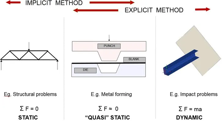
Implicit Analysis
Implicit analysis is a type of static or quasi-static analysis used in FEA. It is well-suited for scenarios where the loading conditions are applied slowly and inertia effects can be neglected. This method is often employed for simulations that involve steady-state or slowly changing conditions, such as thermal stress analysis, creep, and structural stability studies.
- Involves solving a system of equations that includes both the current and later states of the system.
- Can handle larger time steps as stability issues like the explicit method do not limit it.
- Often used for static or quasi-static problems where dynamic effects are not significant.
- Requires the inversion of the stiffness matrix, which can be computationally expensive, especially for large models.
Implicit analysis is also commonly used for nonlinear static and dynamic problems where the response does not change rapidly over time. It is capable of handling complex material behaviours, large deformations, and contact problems, but it typically requires smaller time steps and a more iterative approach to solve the equations governing the system’s behaviour.
In summary, implicit analysis is versatile and can be applied to both linear and nonlinear problems, static or dynamic, provided that the problem does not involve rapid changes that require the fine temporal resolution of an explicit method.
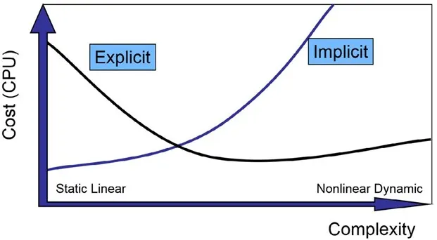
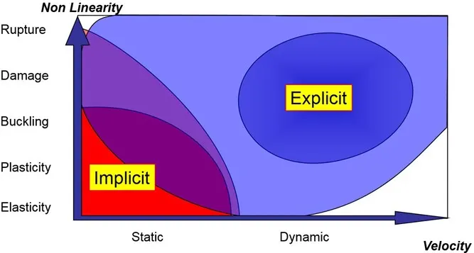
In summary, explicit methods are generally preferred for problems with significant dynamic effects and require small time steps, while implicit methods are suitable for static or slowly varying problems where larger time steps are possible
| Sl No | Explicit Analysis | Implicit Analysis |
| 1 |
Conditionally Stable |
Always Stable |
| 2 |
Time Step Is Small (Microseconds) |
Time Step Is Large (Milliseconds) |
| 3 |
Precision |
Precision |
| 4 |
Diagonal Matrix `[M]^-1` |
Non Diagonal Matrix `([M]+alpha[K])^-1` |
| 5 |
Low Memory (10MW) |
High Memory (6000MW) |
| 6 |
Dynamic And Shock Problems |
Dynamic And Static Problems |
| 7 |
Element-By-Element Method (Local Treatment) |
Global Resolution (Need Of Convergence Of Each Step) |
| 8 |
High Robustness (High And Coupled Nonlinearities) |
Low Robustness (Null Pivots, Divergence....) |
| 9 | Relatively Low Cost (Low CPU, Low Memory) |
Too Expensive (High CPU, High Memory) |
Calculations
The step-by-step solutions for problems using explicit and implicit methods are outlined below.
Given,
`f(u) = u^3+9u^2+4u` -----------------------------------(1)
From the above equation,
`K(u) = (delta(f))/(delta(u)) = 3u^2+18u+4`---------- -(2)
`Delta(F) = KDeltau`---------------------------------------(3)
Regarding the PDF, we also use three equal load increments (or steps) of ∆F.
`DeltaF =1`-------------------------------------------------(4)
Where
`f=` Internal Force`K(u) = K(0)`
`u=` Displacement
`K=` Stiffness
`F=` External Force
`DeltaF =` External Load Increment
`Deltau =` Displacement Increment
1. Explicit Method
The explicit analysis proceeds as follows:
1. Step Number 1
Initially,
`u_0 = 0`
`K(u_0) = K(0) = (3xx0^2)+(18xx0) +4 = 4`
`DeltaF =1`
From (3),
`Deltau_1 = (DeltaF)/(K(u_0)) = 1/4 =0.25`
And,
`u_1=u_0+Deltau_0 = 0+0.25 =0.25`
After the first increments, the following results can be obtained
`(F_"external")_1 = DeltaF = 1`
`(f_"internal")_1 = f(u_1) = 0.25^3+(9xx0.25^2)+(4xx0.25)`
`= 1.5781`
`(F_"external")_1 ne (f_"internal")_1`
Calculating Residue
`R_1 = (f_"internal")_1-(F_"external")_1 = 1.5781-1 = 0.5781`
2. Step Number 2
`u_1 = 0.25`
`K(u_1) = K(0.25) = (3xx0.25^2)+(18xx0.25)+4 = 8.6875`
`DeltaF =1`
From (3),
`Deltau_2 = (DeltaF)/(K(u_1)) = 1/8.6875 =0.1151`
And,
`u_2 = u_1+Deltau_2 = 0.25+0.1151=0.3651`
After two increments, the following results can be obtained
`(F_"external")_2 = DeltaF+DeltaF = 1+1 = 2`
`(f_"internal")_2 = f(u_2) = 0.3651^3+(9xx0.3651^2)+(4xx0.3651)`
`= 2.7087`
`(F_"external")_2 ne (f_"internal")_2`
Calculating Residue
`R_2 = (f_"internal")_2-(F_"external")_2 = 2.7087-2 = 0.7087`
3. Step Number 3
`u_2 = 0.3651`
`K(u_2) = K(0.3651) = (3xx0.3651^2)+(18xx0.3651)+4 = 10.9716`
`DeltaF =1`
From (3),
`Deltau_3 = (DeltaF)/(K(u_2)) = 1/10.9716 =0.09114`
And,
`u_3 = u_2+Deltau_3 = 0.3651+0.09114=0.4562`
After three increments, the following results can be obtained
`(F_"external")_3 = DeltaF+DeltaF+DeltaF = 1+1+1 = 3`
`(f_"internal")_3 = f(u_3) = 0.4562^3+(9xx0.4562^2)+(4xx0.4562)`
`= 3.7298`
`(F_"external")_3 ne (f_"internal")_3`
Calculating Residue
`R_3 = (f_"internal")_3-(F_"external")_3 = 3.7298-3 = 0.7298`
From this,
`F_"external" ne f_"internal"`
This indicates that the external and internal forces are unequal, signifying that they are not in equilibrium.
Following three increments, we are now able to tabulate all the values.
| Step Number (i) | `DeltaF_i` | `Deltau_i` | `u_i` | `(F_"external")_i` | `(f_"internal")_i` |
`R_i = (f_"internal")_i-(F_"external")_i` |
| 1 | 1 | 0.25 | 0.25 | 1 | 1.5781 | 0.5781 |
| 2 | 1 | 0.1151 | 0.3651 | 2 | 2.7087 | 0.7087 |
| 3 | 1 | 0.091114 | 0.4562 | 3 | 3.7298 | 0.7287 |
2. Implicit Method
The implicit analysis proceeds as follows:
`"Tolerance "= 0.01`
1. Step Number 1
Initially,
`u_0 = 0`
`K(u_0) = K(0) = (3xx0^2)+(18xx0) +4 = 4`
`DeltaF =1`
From (3),
`Deltau_1 = (DeltaF)/(K(u_0)) = 1/4 =0.25`
And,
`u_1=u_0+Deltau_1 = 0+0.25 =0.25`
After the first increments, the following results can be obtained
`(F_"external")_1 =(F_"external")_1^0= DeltaF = 1`
`(f_"internal")_1 = (f_"internal")_1^0=f(u_1) = 0.25^3+(9xx0.25^2)+(4xx0.25)`
`= 1.5781`
`(F_"external")_1^0 ne (f_"internal")_1^0`
Calculating Residue
`R_1^"(0)" = (f_"internal")_1^0-(F_"external")_1^0`
`= 1.5781-1`
`= 0.5781>0.01`
The residue values exceed the tolerance level. Therefore, the Newton-Raphson iterations must continue until the residue value falls below the tolerance threshold.
Calculating correction,
`R_1^"(0)" = 0.5781`
`u_1 = u_1^"(0)"=0.25`
`delta(u_1^"(1)") = -[K(u_1^"(0)")]^-1 xxR_1^"(0)"`
`K(u_1^"(0)") = K(0.25)`
`= (3xx0.25^2)+(18xx0.25)+4 = 8.6875`
So,
`delta(u_1^"(1)") = -(8.6875)^-1xx0.5781`
`= -0.06654`
`u_1^"(1)" = u_1^"(0)" +delta(u_1^"(1)")`
`= 0.25+(-0.06654) = 0.18346`
`(F_"external")_1^1 = DeltaF = 1`
`(f_"internal")_1^1 = f(u_1^"(1)")`
`= 0.18346^3+(9xx0.18346^2)+(4xx0.18346)`
`= 1.04293`
Calculating Residue `R_1^"(1)" = (f_"internal")_1^1-(F_"external")_1^1`
`= 1.04293-1`
`=0.04293`
Comparing the value with tolerance
`= 0.04293>0.01` `
The residue values exceed the tolerance level. Therefore, the Newton-Raphson iterations must continue until the residue value falls below the tolerance threshold.
2. Step Number 2
Calculating correction,
`R_1^"(1)" = 0.04293`
`u_1 = u_1^"(1)"=0.18346`
`delta(u_1^"(1)") = -0.06654`
`delta(u_1^"(2)") = delta(u_1^"(1)")-([K(u_1^"(1)")]^-1 xxR_1^"(1)")`
`K(u_1^"(1)") = K(0.18346)`
`= (3xx0.18346^2)+(18xx0.18346)+4 = 7.4032`
So, `delta(u_1^"(2)") = -0.0665-((7.4032)^-1xx0.04293)`
`= -0.07229`
`u_1^"(2)" = u_1^"(0)" +delta(u_1^"(2)")`
`= 0.25+(-0.07229) = 0.17771`
`(F_"external")_1^2 = DeltaF = 1`
`(f_"internal")_1^2 = f(u_1^"(2)")`
`= 0.17771^3+(9xx0.17771^2)+(4xx0.17771)`
`= 1.0006`
Calculating Residue
`R_1^"(2)" = (f_"internal")_1^2-(F_"external")_1^2`
`= 1.0006-1`
`= 0.0006`
Comparing the value with tolerance
`0.0006<0.01`
So we can stop the iteration. The value of displacement is
`u_1 = u_1^"(2)"=0.17771`
3. Step Number 3
Similarly, For the displacement
`u_1 = 0.17771`
`K(u_1) = K(0.17771) = (3xx0.17771^2)+(18xx0.17771)+4 =7.2935`
`DeltaF =1`
From (3),
`Deltau_1 = (DeltaF)/(K(u_1)) = 1/7.2935 =0.1371`
And,
`u_2=u_1+Deltau_1 = 0.17771+0.1371 =0.3148`
After the first increments, the following results can be obtained
`(F_"external")_2 =(F_"external")_2^0= DeltaF +DeltaF = 2`
`(f_"internal")_2 = (f_"internal")_2^0=f(u_2) = 0.3148^3+(9xx0.3148^2)+(4xx0.3148)`
`= 2.1822`
`(F_"external")_2^0 ne (f_"internal")_2^0`
Calculating Residue
`R_2^"(0)" = (f_"internal")_2^0-(F_"external")_2^0`
`= 2.1822-2`
`= 0.1822>0.01`
The residue values exceed the tolerance level. Therefore, the Newton-Raphson iterations must continue until the residue value falls below the tolerance threshold.
Calculating correction,
`R_2^"(0)" = 0.1822`
`u_2 = u_2^"(0)"=0.3148`
`delta(u_2^"(1)") = -[K(u_2^"(0)")]^-1 xxR_2^"(0)"`
`K(u_2^"(0)") = K(0.3148)`
`= (3xx0.3148^2)+(18xx0.3148)+4 = 9.9636`
So, `delta(u_2^"(1)") = -(9.9636)^-1xx0.1822`
`= -0.01828`
`u_2^"(1)" = u_2^"(0)" +delta(u_2^"(1)")`
`= 0.3148+(-0.01828) = 0.2965`
`(F_"external")_2^1 = DeltaF = 2`
`(f_"internal")_2^1 = f(u_2^"(1)")`
`= 0.2965^3+(9xx0.2965^2)+(4xx0.2965)`
`= 2.0032`
Calculating Residue
`R_2^"(1)" = (f_"internal")_2^1-(F_"external")_2^1`
`= 2.0032-2`
`=0.0032`
Comparing the value with tolerance
`= 0.0032<0.01`
We can stop the iteration. The value of displacement
`u_2 = u_2^"(1)"=0.2965`
4. Step Number 4
Similarly, For the displacement
`u_2 = 0.2965`
`K(u_2) = K(0.2965) = (3xx0.2965^2)+(18xx0.2965)+4 =9.6007`
`DeltaF =1`
From (3),
`Deltau_2 = (DeltaF)/(K(u_2)) = 1/9.6007 =0.1041`
And,
`u_3=u_2+Deltau_2 = 0.2965+0.1041 =0.4006`
After the first increments, the following results can be obtained
`(F_"external")_3 =(F_"external")_3^0= DeltaF +DeltaF +DeltaF = 3`
`(f_"internal")_3 = (f_"internal")_3^0=f(u_3) = 0.4006^3+(9xx0.4006^2)+(4xx0.4006)`
`= 3.111`
`(F_"external")_3^0 ne (f_"internal")_3^0`
Calculating Residue
`R_3^"(0)" = (f_"internal")_3^0-(F_"external")_3^0`
`= 3.111-3`
`= 0.111>0.01`
The residue values exceed the tolerance level. Therefore, the Newton-Raphson iterations must continue until the residue value falls below the tolerance threshold.
Calculating correction,
`R_3^"(0)" = 0.111`
`u_3 = u_3^"(0)"=0.4006`
`delta(u_3^"(1)") = -[K(u_3^"(0)")]^-1 xxR_3^"(0)"`
`K(u_3^"(0)") = K(0.4006)`
`= (3xx0.4006^2)+(18xx0.4006)+4 = 11.6922`
So, `delta(u_3^"(1)") = -(11.6922)^-1xx0.111`
`= -0.00949`
`u_3^"(1)" = u_3^"(0)" +delta(u_3^"(1)")`
`= 0.4006+(-0.00949) = 0.3911`
`(F_"external")_3^1 = DeltaF +DeltaF+DeltaF= 3`
`(f_"internal")_3^1 = f(u_3^"(1)")`
`= 0.3911^3+(9xx0.3911^2)+(4xx0.3911)`
`= 3.0008`
Calculating Residue
`R_3^"(1)" = (f_"internal")_3^1-(F_"external")_3^1`
`= 3.0008-3`
`=0.0008`
Comparing the value with tolerance
`= 0.0008<0.01`
So we can stop the iteration. The value of displacement is
`u_3 = u_3^"(1)"=0.3911`
we are now able to tabulate all the values.
| Step Number (i) | `DeltaF_i` | `|Deltau_i|` | `u_i` | `(F_"external")_i` | `(f_"internal")_i` |
`R_i = (f_"internal")_i-(F_"external")_i` |
| 1 | 1 | 0.07229 | 0.1777 | 1 | 1.0006 | 0.0006 |
| 2 | 1 | 0.01828 | 0.2965 | 2 | 2.0032 | 0.0032 |
| 3 | 1 | 0.00949 | 0.3911 | 3 | 3.0008 | 0.0008 |
The scatter plot is done using WPS Office.
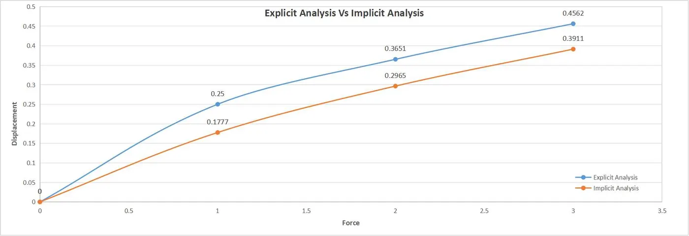
Conclusions
- The explicit method does not account for any tolerance values, which means the values obtained from the analysis may contain errors. There is no need for stiffness matrix inversions or other iterative methods. Essentially, it requires minimal CPU memory, which significantly speeds up the process.
- In the implicit method, the tolerance value is considered and compared in each iteration. The process continues until the residue is less than the tolerance, resulting in more precise values. However, due to these iterations and inversions of the stiffness matrix, it requires significantly more CPU memory, which impacts the speed of analysis.