Week - 2 - Explicit and Implicit Analysis

OBJECTIVE:

• To understand the mathematical concept behind the Implicit and Explicit methods which is used in finite element analysis.
• Solve a non-linear equation using both methods and plot their graph.

INTRODUCTION:

Explicit Analysis

• It is used in dynamic analysis such as crash test, drop test.
• In this method result for current step is calculated.
• This method does not consider equilibrium of the forces.
• In Explicit analysis critical time is important. Therefore it is conditionally stable.
• This method is used in large deformation analysis such as car crash test.

Implicit Analysis:

• It is mainly used in static analysis.
• In this method result for next step is calculated.
• This method considers equilibrium of the forces by converging the residual close to zero using iteration method.
• For this analysis time does not matter.
• This method is used when there is small deformation over longer duration.

                                                                                   Non-linear static problem:

• Consider the case of a simple bar in tension, where force in the bar is a non-linear function of the displacement.
• Given, `f(u)=u^3+9u^2+4u`
• Here the variables used are u for displacement, f for internal force int the bar, F for external load applied on the bar and k for the stiffness.
• `DeltaF= kDeltau`

                                                                                                                                                                                                                                    

Explicit Approach:

We will be considering three equal increments of ΔF=1. 

df=k(u).du

`f(u)=u^3+9u^2+4u`

`k(u)=(df)/(du)`

⇒ k(u)= `3u^2+18u+4`

Step 1: u₀=0

⇒ k(u₀)= `3u_0^2+18u_0+4`= 4

⇒ Δu₁= `(DeltaF)/(k(u_0))`= `1/4`

⇒ `u_1`= `u_0+Deltau_1`= 0.25

Step 2: 

`k(u_1)= 3u_1^3+9u_1^2+4u_1`= 8.687

Δu₂= `(DeltaF)/(k(u_1))`= `1/8.6875`

`u_2= u_1+Δu_2`= 0.365

Step 3:

`k(u_2)= 3u_2^3+9u_2^2+4u_2`= 10.969675`

`Deltau_3`= `(DeltaF)/(k(u_2))`= `1/10.96975`

`u_3= u_2+Δu_3`= 0.456

From the above three steps, the following summary of explicit analysis is obtained:

Step i	ΔFi	Δui	ui	(Fext)i	(fint)i	fint-Fext= R
1	1.0	0.25	0.25	1.0	1.578	0.578
2	1.0	0.115	0.365	2.0	2.707	0.707
3	1.0	0.0911	0.456	3.0	3.792	0.792

Implicit Approach:

To achieve equilibrium between external and internal force, Newton-Raphson iterations are used to minimise the Residual, R(u).

The tolerance is taken as 0.01

We will be considering three equal increments of ΔF=1. 

df=k(u).du

`f(u)=u^3+9u^2+4u`

`k(u)=(df)/(du)`

⇒ k(u)= `3u^2+18u+4`

Step 1:

u₀=0

⇒ k(u₀)= `3u_0^2+18u_0+4`= 4

⇒ Δu₁= `(DeltaF)/(k(u_0))`= `1/4`

⇒ `u_1`= `u_0+Deltau_1`= 0.25

⇒ `k(u_1)= 3u_1^3+9u_1^2+4u_1`= 8.687

⇒ f_int= `(u_1)^3+9(u_1)^2+4(u_1)`= 1.578

Residual check, `R^((0))`= f_int-F_ext= 0.578 (>0.01 tolerance)

Correction for `u_1`= `u_1^((0))`

`deltau^((1)) = -[k(u_1^((0)))]^-1*R^((0))`= -0.066

⇒`u_1^((1))= u_1^((0))+deltau^((1))`= 0.184

⇒ `k(u_1)= 3u_1^3+9u_1^2+4u_1`= 7.4135

⇒ f_int= `(u_1^((1)))^3+9(u_1^((1)))^2+4(u_1^((1)))`= 1.0469

Residual check, `R^((1))`= f_int-F_ext= 0.046 (>0.01 tolerance)

Correction for `u_1`= `u_1^((0))` 

`deltau^((2)) = deltau^((1))-[k(u_1^((1)))]^-1*R^((1))`= -0.0722

⇒`u_1^((2))= u_1^((0))+deltau^((2))`= 0.1778

⇒ f_int= `(u_1^((2)))^3+9(u_1^((2)))^2+4(u_1^((2)))`= 1.0013

Residual check, `R^((2))`= f_int-F_ext= 0.0013 (<0.01 tolerance)

⇒ `u_1= u_1^((2))= 0.1778`

Step 2:

`k(u_1)= 3u_1^3+9u_1^2+4u_1`= 7.2176

⇒ Δu₂= `(DeltaF)/(k(u_1))`= `1/7.21726`= 0.13855

⇒ `u_2= u_1+Δu_2`= 0.3163

⇒ `k(u_2)= 3u_2^3+9u_2^2+4u_2`= 9.9935

⇒ f_int= `(u_2)^3+9(u_2)^2+4(u_2)`= 2.19725

Residual check, `R^((0))`= f_int-F_ext= 0.19725 (>0.01 tolerance)

Correction for `u_2`= `u_2^((0))`

`deltau^((1)) = -[k(u_2^((0)))]^-1*R^((0))`= -0.01973

⇒ `u_2^((1))= u_2^((0))+deltau^((1))`= 0.2965

⇒ f_int= `(u_2^((1)))^3+9(u_2^((1)))^2+4(u_2^((1)))`= 2.003276

Residual check, `R^((1))`= f_int-F_ext= 0.003 (<0.01 tolerance)

⇒ `u_2= u_2^((1))= 0.2965`

Step 3:

`k(u_2)= 3u_2^3+9u_2^2+4u_2`= 9.600736

⇒ Δu₃= `(DeltaF)/(k(u_2))`= `1/9.600736 = 0.104158`

⇒`u_3= u_2+Δu_3`= 0.400658

⇒ `k(u_3)= u_3^3+9u_3^2+4u_3`= 11.6934

f_int= `(u_3)^3+9(u_3)^2+4(u_3)`= 3.111689

Residual check, `R^((0))`= f_int-F_ext= 0.111689 (>0.01 tolerance)

Correction for `u_3`= `u_3^((0))`

`deltau^((1)) = -[k(u_3^((0)))]^-1*R^((0))`= -0.00955

`u_3^((1))= u_3^((0))+deltau^((1))`= 0.3911

f_int= `(u_3^((1)))^3+9(u_3^((1)))^2+4(u_3^((1)))`= 3.00085

Residual check, `R^((1))`= f_int-F_ext= 0.00085 (<0.01 tolerance)

⇒ `u_3= u_3^((1))= 0.3911`

From the above three steps, the following summary of implicit analysis is obtained:

Step i	ΔFi	ui	(Fext)i	(fint)i	fint-Fext= R
1	1.0	0.1778	1.0	1.0013	0.0013
2	1.0	0.2965	2.0	2.0032	0.0032
3	1.0	0.3911	3.0	3.0008	0.0008

Solving the relation,`f(u)=u^3+9u^2+4u`  the following summary of exact values are obtained:

ΔF	ui
1	0.17761
2	0.29615
3	0.39102

RESULT:

CONCLUSION:

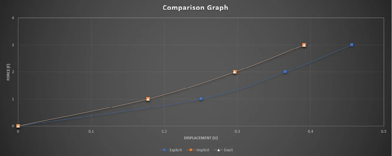
• From the above graph plotted using F and u values, it is observed that the implicit analysis of the three increments in force follows closer to the exact values.
• Whereas the explicit analysis deviates away from the exact values. This is due to residual (R) which indicates non-equilibrium between internal force and external load at each increment step. 
• The Newton-Raphson iterations converged the residual to the required tolerance which resulted in better values in implicit method.
• The comparison of both calculation methods points out the complexity of Implict method.