Week - 2 - Explicit and Implicit Analysis
AIM:
To solve F(u) = u3+9u2+4u using both Explicit and Implicit Methods ( have a tolerance of 0.001).
COMPARISON BETWEEN IMPLICIT AND EXPLICT:
Explicit and implicit methods are used in numerical analysis for finding numerical approximations to solve solutions of time-dependent ordinary and partial differential equations which require computer simulations of physical processes.
| IMPLICIT | EXPLICIT | |
| DEFORMATION | SMALL | LARGE |
| WHAT CAUSES LARGE DEFORMATION | PURE FORCE | VELOCITY/ACCELERATION WITH MASS AND INERTIA |
| K MATRIX INVERSE | YES | NO |
| TIME STEP SIZE | LARGE | SMALL |
| COST PER TIME STEP | LARGE | SMALL |
PROCEDURE:
| Explicit Method: | ||||||
| f(u) = u3 + 9u2 + 4u | ||||||
| Stiffness of the bar is given by k(u) | ||||||
| k(u) = (d f(u))/(dx) = 3u2 + 18u + 4 | ||||||
| Step 1 | ||||||
| ΔF=1, u0=0.0 | ||||||
| K (u0) = 3(0)2 +18(0) + 4 | ||||||
| = 4 | ||||||
| Now Δu1 = ΔF/k(u=0) = ¼ = 0.25 | ||||||
| u1 = u + Δu1 = 0 + 0.25 = 0.25 | ||||||
| F (u1 = 0.25) = (0.25)3 + 9(0.25)2 + 4(0.25) = 0.015625 + 9(0.0625) +1 = 1.578 | ||||||
| Residual R1 = F (u1) – ΔF = 1.578 – 1 = 0.578 | ||||||
| Step 2 - ΔF =1; u = 0.25 | ||||||
| K (u = 0.25) = 3(0.25)2 +18(0.25) + 4 = 0.1875 + 4.5 + 4 | ||||||
| = 8.6875 | ||||||
| Now Δu2 = ΔF/k(u=0) = 1/8.6875= 0.1151 | ||||||
| u2 = u1 + Δu2 = 0.25 + 0.1151 = 0.3651 | ||||||
| F (u2 = 0.3651) = (0.3651)3 + 9(0.3651)2 + 4(0.3651) = 0.0487 + 1.2 + 1.46 | ||||||
| = 2.709 | ||||||
| Residual R2 = F (u2) – ΔF = 2.709 – 2 = 0.709 | ||||||
| Step 3 - ΔF =1; u = 0.365 | ||||||
| K (u = 0.365) = 3(0.365)2 +18(0.365) + 4 = 0.4 + 6.57 + 4 | ||||||
| = 10.97 | ||||||
| Now Δu3 = ΔF/k(u=0) = `1/10.97`= 0.091 | ||||||
| u3 = u2 + Δu3 = 0.365 + 0.091 = 0.456 | ||||||
| F (u3 = 0.456) = (0.456)3 + 9(0.456)2 + 4(0.456) = 0.095 + 1.871 + 1.824 | ||||||
| = 3.79 | ||||||
| Residual R3 = F (u3) – ΔF = 3.79 – 3 = 0.79 | ||||||
| Fext = 3, fint = 3.79 | ||||||
| Thus, Fext ≠ fint. | ||||||
| Step | ΔFi | Δui | ui | (Fext)i | (fint)i | Ri |
| 1 | 1 | 0.25 | 0.25 | 1 | 1.578 | 0.578 |
| 2 | 1 | 0.1151 | 0.365 | 2 | 2.709 | 0.709 |
| 3 | 1 | 0.091 | 0.456 | 3 | 3.79 | 0.79 |
| Implicit Method: | ||||||
| Tolerance = 0.001 | ||||||
| F(u) = u3 + 9u2 + 4u | ||||||
| ΔF = KΔu | ||||||
| K(u) = `(d F(u))/(du)` = 3u2 + 18u + 4 | ||||||
| Step 1 – Initial condition ΔF =1; u = 0 | ||||||
| K (u = 0) = 3(0)2 +18(0) + 4 | ||||||
| = 4 | ||||||
| Now Δu1 = ΔF/k(u=0) = ¼ = 0.25 | ||||||
| u1 = u + Δu1 = 0 + 0.25 = 0.25 | ||||||
| F (u1 = 0.25) = (0.25)3 + 9(0.25)2 + 4(0.25) = 0.015625 + 9(0.0625) +1 = 1.578 | ||||||
| Residual R0 = F (u1) – ΔF = 1.578 – 1 = 0.578 | ||||||
| Since ||R0 || > 0.001 | ||||||
| Since residual value is grater that tolerence, another Newton-Raphson iteration is necessary. | ||||||
| Calculate the correction to u1(0) = u1 =0.25 | ||||||
| K (u1(0) = 0.25) = 3(0.25)2 +18(0.25) + 4 = 0.1875 + 4.5 + 4 | ||||||
| = 8.6875 | ||||||
| δu1 = - [K (u10)]-1 x R(0) = - (8.6875)-1 x0.578 = - 0.0665 | ||||||
| u1(1) = u1(0) + δu1 = 0.25 + (-0.0665) = 0.1835 | ||||||
| F (u1(1) = 0.1835) = (0.1835)3 + 9(0.1835)2 + 4(0.1835) = 0.006 + 0.303 + 0.734 | ||||||
| = 1.043 | ||||||
| Residual R(1) = F (u1(1)) – ΔF = 1.043 – 1 = 0.043 | ||||||
| Since ||R(1) || > 0.001 | ||||||
| Since residual value is grater that tolerence, another Newton-Raphson iteration is necessary. | ||||||
| Calculate the correction | ||||||
| K (u1(1) = 0.25) = 3(0.1835)2 +18(0.1835) + 4 = 0.101 + 3.303 + 4 | ||||||
| = 7.404 | ||||||
| δu2 = δu1 - [K (u1(0))]-1 R0 = -0.0665 - (7.404)-1 x0.043 = - 0.0723 | ||||||
| u1(2) = u1 + δu2 = 0.25 + (-0.0723) = 0.1777 | ||||||
| F (u1(2) = 0.1777) = (0.1777)3 + 9(0.1777)2 + 4(0.1777) = 0.0056 + 0.284 + 0.7108 | ||||||
| = 1.0004 | ||||||
| Residual R1 = F (u1(2)) – ΔF = 1.0004 – 1 = 0.0004 | ||||||
| Since ||R1 || < 0.001 | ||||||
| No further iterations are necessary. | ||||||
| So u1 = 0.1777 & F (u1) = 1.0004 | ||||||
| Step 2 - ΔF =1; u = 0.1777 | ||||||
| K (u = 0.1777) = 3(0.1777)2 +18(0.1777) + 4 = 0.094 + 3.1986 + 4 = 7.2926 | ||||||
| Now Δu2 = ΔF/k(u=0.1777) = 1/7.2926 = 0.1371 | ||||||
| u2 = u1 + Δu2 = 0.1777 + 0.1371 = 0.315 | ||||||
| F (u2 = 0.315) = (0.315)3 + 9(0.315)2 + 4(0.315) =0.03125 + 0.893 +1.26 = 2.184 | ||||||
| Residual R0 = F (u2) – ΔF = 2.184 – 2 = 0.184 | ||||||
| Since ||R0 || > 0.001 | ||||||
| Since residual value is grater that tolerence, another Newton-Raphson iteration is necessary. | ||||||
| Calculate the correction to u2(0) = u2 | ||||||
| K (u2(0) = 0.315) = 3(0.315)2 +18(0.315) + 4 = 0.297 + 5.67 + 4 | ||||||
| = 9.967 | ||||||
| δu2 = - [K (u2(0))]-1 R0 = - (9.967)-1 x0.184 = - 0.0184 | ||||||
| u2(1) = u2(0) + δu2 = 0.315 + (-0.0184) = 0.296 | ||||||
| F (u2(1) = 0.296) = (0.296)3 + 9(0.296)2 + 4(0.296) = 0.026 + 0.788 + 1.184 | ||||||
| = 1.998 | ||||||
| Residual R1 = F (u2(1)) – ΔF = 1.998 – 2 = - 0.002 | ||||||
| Since ||R1 || > 0.001 | ||||||
| Since residual value is grater that tolerence, another Newton-Raphson iteration is necessary. | ||||||
| So u2 = 0.296 & F (u2) = 1.998 | ||||||
| Step 3 - ΔF =1; u = 0.296 | ||||||
| K (u = 0.296) = 3(0.296)2 +18(0.296) + 4 = 0.262 + 5.328 + 4 = 9.59 | ||||||
| Now Δu3 = ΔF/k(u=0.296) = 1/9.59 = 0.104 | ||||||
| u3 = u2 + Δu3 = 0.296 + 0.104 = 0.4 | ||||||
| F (u3 = 0.4) = (0.4)3 + 9(0.4)2 + 4(0.4) =0.064 + 1.44 +1.6 = 3.104 | ||||||
| Residual R0 = F (u2) – ΔF = 3.104 – 3 = 0.104 | ||||||
| Since ||R0 || > 0.001 | ||||||
| Since residual value is grater that tolerence, another Newton-Raphson iteration is necessary. | ||||||
| Calculate the correction to u3(0 )= u3 | ||||||
| K (u3(0 ) = 0.4) = 3(0.4)2 +18(0.4) + 4 = 0.48 + 7.2 + 4 | ||||||
| = 11.68 | ||||||
| δu3 = - [K (u3(0 ))]-1 xR0 = - (11.68)-1 x0.104 = - 0.009 | ||||||
| u3(1) = u3(0 ) + δu3 = 0.4 + (-0.009) = 0.391 | ||||||
| F (u3(1) = 0.391) = (0.391)3 + 9(0.391)2 + 4(0.391) = 0.06 + 1.376 + 1.564 | ||||||
| = 3 | ||||||
| Residual R1 = F (u3(1)) – ΔF = 3 – 3 = 0 | ||||||
| Since ||R1 || < 0.001 | ||||||
| No further iterations are necessary. | ||||||
| So u3 = 0.391 & F (u3) = 3 | ||||||
| Step | ΔFi | ui | (Fext)i | (fint)i | Ri | |
| 1 | 1 | 0.1777 | 1 | 1.0004 | 0.0004 | |
| 2 | 1 | 0.296 | 2 | 1.998 | -0.002 | |
| 3 | 1 | 0.391 | 3 | 3 | 0 | |
| EXACT VALUES | ||||||
| F(u) | u | |||||
| 1 | 0.1776 | |||||
| 2 | 0.2962 | |||||
| 3 | 0.391 | |||||
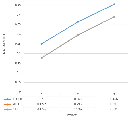
PLOT:
CONCLUSION:
It is evident from the results that the explicit analysis drifts from the true solution. Whereas implicit comes closer to the exact solution. The plot also shows that the implicit method has less error when compared to the explicit method, but it is a time-consuming process – explicit method can predict approx. solutions much faster with repeated iterations.