Week - 2 - Explicit and Implicit Analysis

Aim-

To study the Implicit and explicit analysis methods and how so solve problems using both the methods mathematically.

Theory-

What Is Implicit Method-

   Implicit analysis works by trying solutions or iterations in attempts to establish static equilibrium (within a certain tolerance) with respect to the loading or displacement applied. We are solving for unknown displacements through matrix inversion. When the problem is nonlinear in any way – we think of geometry, material, contact – the solution is obtained over a number of small increments and the solution for the current increment is based upon the result from the previous one (and so on). When we have large models or significant nonlinearity, inverting the matrix is highly computationally expensive and sometimes impossible. When solutions can be found, they are unconditionally stable and allow reasonably large chunks of ‘time’ (although it’s more like chunks of displacement) to be solved for at once.

When to use Implicit?

Implicit methods should be used when the boundary conditions affect the structure slowly, and the effects of strain rates are minimum. Once the increment of stress as a function of strain can be established, geometry can be analysed using implicit methods.

The global equilibrium in the model is established in each time increment. This means each increment has to converge.

After global equilibrium is converged, solver calculates all the local finite element variables (stresses, strain, etc.) for each increment.

• Pros: Since global equilibrium is verified at each time increments, those increments can be large.
• Cons: Each time, increments are computed slowly and needed to get to the global equilibrium.

What Is Explicit Method-

   Explicit solvers, on the other hand, solve for acceleration. No iterations are required because nodal accelerations are calculated directly. We are taking the kinematic conditions from one small increment of time and using them to calculate those conditions at the next. Hence, the state at the end of the increment in question is based only upon the displacements, velocities and accelerations at the beginning of that same increment. What has gone previously is irrelevant and convergence is a non-issue.

When to use Explicit?

 Explicit methods should be used when the strain rates is equal to 10^-3 per second or more. These events can be illustrated by some examples such as an automotive crash, ballistic explosion, drop and so on. In these cases, besides the variation of stress with strain, the rate of strain also needs to be considered.

There are no convergence criteria to check or iteration. The solver focus the calculation of local finite element variables.

Solver calculates all of the local finite element variables for given incrementation, and move to the next one.

• Pros: Each increment is calculated extremely fast.
• Cons: The time step has to be super small. Otherwise, it’s impossible to pursue this equilibrium.

Procedure-

• We will solve the given equation by borh methods mathematically one by one.

                                            F(u)=u³+9u²+4u

Explicit Method-

F(u)=u³+9u²+4u………………………………………………………………………………………………………………. (1)

From (1) it follows that the stiffness of the bar is,

K(u)=dF/du=3u²+18u+4…………………………………………………………………………………………………... (2)

For explicit dynamics solution-

Step-1-

At u=0, equation (2) becomes.

K(u₀) =3*0²+18*0+4=4, ΔF=1, so,

Δu₁=ΔF/K(u₀) = 1/4=0.25

u₁₌ u₀+ Δu₁ = 0+0.25 = 0.25

Step-2-

At u₁=0.25, equation (2) becomes.

K(u₁) =3*0.25²+18*0.25+4=8.6875, ΔF=1, so,

Δu₂=ΔF/K(u₁) = 1/8.6875=0.1151

u₂₌ u₁+ Δu₂ = 0.25+0.1151 = 0.3651

Step-3-

At u₂=0.3651, equation (2) becomes.

K(u₂) =3*0.3651²+18*0.3651+4=10.9717, ΔF=1, so,

Δu₃=ΔF/K(u₂) = 1/10.9717=0.09114

u₃₌ u₁+ Δu₃ = 0.3651+0.09114=0.4562

Finally, from the three steps the following results are obtained.

Now, we will check whether the solution obtained is in equilibrium or not,

F_ext = ∆F + ∆F + ∆F = 3.0

From equation (1),

F_int= (0.4562)³+9(0.4562)²+4(0.4562)

     =3.7928

It is evident from the results that external and internal forces are NOT in equilibrium because F_ext ≠ F_int. Table 1 summarizes the main results for the explicit analysis.

Table 1: Summary of explicit analysis results

Step i	ΔFi	Δui	ui	(Fext)i	(Fint)i	Fint-Fext=R
1	1.0	0.25	0.25	1	1.578	0.578
2	1.0	0.1151	0.3651	2	2.708	0.708
3	1.0	0.09114	0.4562	3	3.7928	0.7928

Implicit Method-

F(u)=u³+9u²+4u………………………………………………………………………………………………………………. (1)

From (1) it follows that the stiffness of the bar is,

K(u)=dF/du=3u²+18u+4…………………………………………………………………………………………………. (2)

Implicit transient analysis has no inherent limit on the size of the time step. As such, implicit time steps are generally several orders of magnitude larger than explicit time steps. 

  where u= displacement, f= internal force in bar, F= external force in bar 

   ∆u = incremental displacements, ∆F = incremental external applied forces.

   using relation, ∆F = k*∆u, Tolerance= 10^-2

  Step 1:

  Take u₀=0,

  (2) ≥ k(u₀) =3(0)²+18x0+4 = 4

  now, ∆u₁ = ∆F/k(u₀) = 1/4 = 0.25

  u₁ = u₀+∆u₁= 0.25

  Checking residual, R

  F_ext=∆F=1     f(int) = (0.25)³+(9x (0.25)²) + (4x0.25) =1.578

  R0 = 1.578-1 = 0.578 > 10^-2

  So, Newton-Raphson iterations are necessary.

  calc. the correction to u₁=u₁(0)

   ẟu ⁽¹⁾ = -[k(u₁⁽⁰⁾]^-1 x R ⁽⁰⁾ = -[(3x0.25²) +(18x0.25) +4]^-1 x 0.578 = -0.0665

  updated, u₁⁽¹⁾ = u₁⁽⁰⁾ + ẟu⁽¹⁾ = 0.25-0.0665 = 0.1835

  Check residual again, R₁,

  F_ext = 1, F_int = (0.1835)³+((9x (0.1835)²) + (4x0.1835) = 1.0432

  R¹ = 1.0432-1 = 0.0432 > 10^-2, another Newton-Raphson iteration needed.

  Calc. the correction to u₁ = u₁⁽¹⁾,

  ẟu⁽²⁾ = ẟu⁽¹⁾-[k(u₁⁽¹⁾]^-1 x R¹ = (-0.0665)-(8.6875)^-1 x(0.0432) = -0.0714

  updated, u1(2) = u₁⁽¹⁾ + ẟu⁽²⁾ = 0.25-0.0714 = 0.1786

  Checking Residual again R₂,

  F_ext=1, F_int= (1) ≥ (0.1786)³+(9x0.1786²) +(4x0.1786) = 1.0071

  R² = 1.0071-1 = 0.0071 < 10^-2

  Therefore, no iterations needed, final u₁ = 0.1786.

  Step 2:

    Take u₁=0.1786, equation (2) becomes,

  k(u₁) =3(0.1786)²+18x0.1786+4 = 7.31

  now, ∆u₂ = ∆F/k(u₁) = 1/7.31 = 0.1368

  u₂ = u₁+∆u₂= 0.1786+0.1368=0.3154

  Checking residual, R

  F_ext=∆F=2    f(int) = (0.3154)³+(9x (0.3154)²) + (4x0.3154) =2.188

  R₀ = 2.188-2 = 0.188 > 10^-2

  So, Newton-Raphson iterations are necessary.

  calc. the correction to u₁=u₁(0)

   ẟu ⁽¹⁾ = -[k(u₂⁽⁰⁾)]^-1 x R ⁽⁰⁾ = -[(3x0.3154²) +(18x0.3154) +4]^-1 x 0.188 = -0.0188

  updated, u₂⁽¹⁾ = u₂⁽⁰⁾ + ẟu⁽¹⁾ = 0.3154-0.0188 = 0.2966

  Check residual again, R¹,

  F_ext = 2, F_int = (0.2966)³+((9x (0.2966)²) + (4x0.2966) = 2.004

  R¹ =2.004-2 = 0.004 < 10^-2

  Therefore, no iterations needed, final u₂ = 0.2966.

  Step 3:

  similarly, as step 1, we get u₃=0.3911.

The results of the implicit analysis are summarized in Table 2. It is evident from the table that the external forces and internal forces are coming into equilibrium.

Table 2: Summary of implicit analysis results

Step i	ΔFi	Δui	ui	(Fext)i	(Fint)i	Fint-Fext=R
1	1	0.25	0.1786	1	1.0071	0.0071
2	1	0.1374	0.2966	2	2.0042	0.0042
3	1	0.1041	0.3911	3	3.0008	0.0008

 

Exact values:

     Take, F(u)= u3+9u2+4u = 1 

     using Scientific calculator, we get u=0.1776

     take, F(u)= u3+9u2+4u = 2

     using Scientific calculator, we get u= 0.2962

    take, F(u)= u3+9u2+4u = 3

    using Scientific calculator, we get u= 0.3910

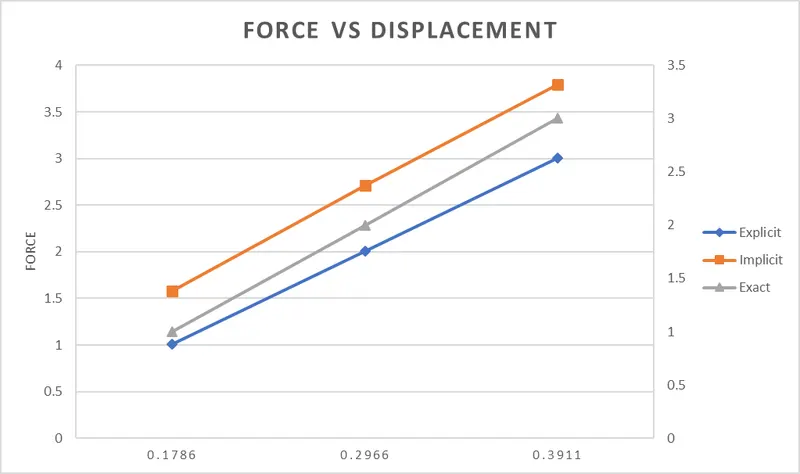
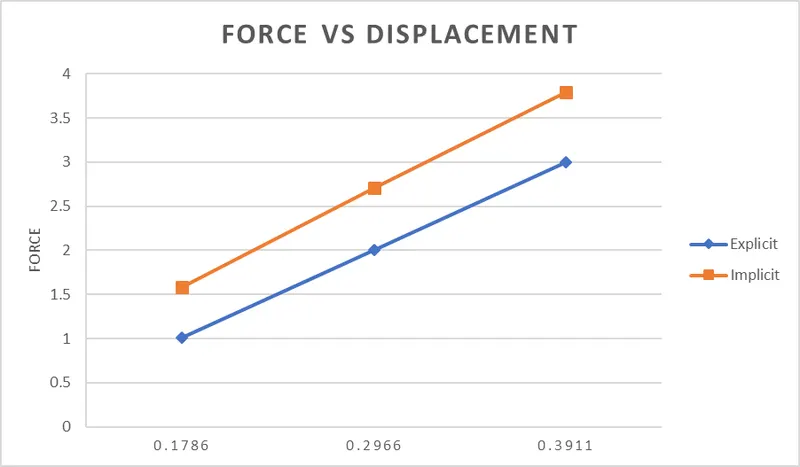
• From above graphical data we can say that the explicit method drift from exact solution and lacks to achieve the equilibrium condition in between external and internal forces.
• To achieve  exact equilibirum condition we used implicit method and using Newton-Raphson Method we have converged to exact solution with minimum residual difference in both forces which may be neglected letter.

Conclusion-

• The implicit solver is really useful if conditions in analysis happen relatively slow. Ideal analyses are generally longer than 1 second. The advantage is that the time increment can be set as big as users want.
• Implicit Solver method is used for, Unknown x is found by inversion of stiffness matrix (K), Newton-Raphson / Enforced equilibrium solutions., More accurate,
• Disadvantages-Extremely time-consuming for large models, Requires more computer storage.
• Good decision for structure dynamic types which load rates are slow;
  – Slowly applied displacements
  – Low frequency response
  – Vibration
  – Oscillation

• The explicit solver is great for fast events (mostly less than 0.1 second) Explicit solver calculates how big the time increment should be and set the time increment. The speed of sound in material properties depends on density of material. This is called “mass scaling”. The time step in explicit method depends on the mesh (element size and element quality), young's modulus, and density.

• Unknown x is found by inversion of mass matrix (M), Direct solutions, Central difference methods are used.
• Computationally efficient for large models with short dynamic response time, Requires less computer storage.
• Disadvantage-Less accurate.
• Good decision for structure dynamic types which are wave propagation;
  – Car crash
  – Blast effect
  – Drop
  – Metal stamping

• A nonlinear analysis is illustrated using an incremental explicit and implicit procedure. The results are plotted for comparison. It is evident from the results that the explicit analysis drifts from the true solution. To overcome this problem an implicit analysis is used, which includes Newton-Raphson iterations to enforce equilibrium between internal and external forces. The techniques demonstrated are for a load control scheme.
• Above example is very useful for understanding the solution method for non-linear problem and how expicit and implicit methods are used.