Week - 2 - Explicit and Implicit Analysis

Explicit and Implicit Analysis

OBJECTIVE:-

To explain Explicit and Implicit Methods of solving problem in FEA in detail and to solve given equation using both Explicit and Implicit Methods.

EXPLANATION:-

Implicit and Explicit Methods:-

Implicit and Explicit are two types of approaches that can be used to solve the finite element problem. The implicit approach is useful in problems in which time dependency of the solution is not an important

factor e.g. static structural, harmonic, modal analysis, etc. whereas the Explicit Dynamics approach is most helpful in solving high deformation time-dependent problems such as Crash, Blast, Impact, etc.

Implicit Method:-

One method of solving for the unknowns is through matrix inversion or equivalent processes. This is known as an implicit analysis. When the problem is nonlinear, the solution is obtained in a number of steps

and the solution for the current step is based on the unknowns of current steps as well as known solution from the previous step. For large models, inverting the matrix is highly expensive and will require

advanced iterative solvers over standard direct solvers.

These solutions are unconditionally stable and facilitate larger time steps. So it is suitable for problems that tend to be high linear, static and quasi-static but despite this advantage, the implicit methods can be

extremely time-consuming when solving dynamic and nonlinear problems due to iterations performed in order to achieve the global equilibrium for each time step.

Implicit methods are mainly used in softwares such as Ansys, Nastran, Abaqus etc.

Explicit Method:-

Explicit analyses aim to solve for acceleration. In most cases, the mass matrix is considered as a diagonal matrix. Inversion of a diagonal matrix is straightforward and includes inversion of the terms on the

diagonal only. In these calculations, solutions are not unconditionally stable and thus smaller time steps are required.

In this method, the solution for the current step is based on the known solution from the previous step.

These solutions are not unconditionally stable and so does not facilitate larger time steps that's why time step has to be very small.

Explicit methods specially used for solving problems such as Crash, Impact, Penetration etc.

Essence of Implicit Method of Solving:-

Firstly, in each time increment the “global equilibrium” in the model is established. This means that each increment has to converge and only after global equilibrium is established, solver calculates all the local

finite element variables (stresses etc.) for this increment. It is a kind of iterative process which anyhow tries to establish the equilibrium, no matter what number of iterations it has to perform for achieving the

same.

Benefits: Since global equilibrium is verified at each time increments, those increments can be big.

Drawbacks: Each time increment computes slowly, since iterations are needed to get to the global equilibrium.

Essence of Explicit Method of Solving:-

It works in a way, that converge each step is not needed. There are no convergence criteria to check and no iterations unlike implicit method and Instead of verifying the “global equilibrium”, solver assumes that

the equilibrium “simply exists”. This means that the solver goes straight into calculation of local finite element variables as such procedure has only one step so it calculate all of the local finite element variables

for given increment, and move to the next one.

Benefits: Each increment calculates extremely fast.

Drawbacks: For this to work, the time step has to be extremely small. Otherwise, it’s impossible to maintain this equilibrium that is assumed to “simply exist”. To achieve this, user do not have direct control over

how big time increments explicit solver will take and solver itself calculates how small timesteps are still needed but infact those acceptable time increments are super small. This is why explicit problems should

last fractions of the second but If they would last seconds, it would need millions of increments.

Calculation-:

Function Given - F(u) = u3+9u2+4u

Explicit method:-

F(u) = u3+9u2+4u (1)

For stiffness ,

K(u)= dF(u)/du = 3u^2+18u+4 (2)

From equ (1) and (2),

∆F = k∆u (3)

Step-1

For initial condition, ΔF=1

The value of u(0)=0

Now, substituting in equation (2)

K(0)= 3(0)^2+18(0)+4

K(0)=4

Then from equation (3) implies,

Δu(1) = ∆F/k(0) = 1/4 = 0.25

and also from u(1)=u(0)+Δu(1) = 0+0.25

u(1)=0.25

Step-2

Consider u(1)=0.25 then

K(1) = 3(0.25)^2+18(0.25)+ 4

K(1)=8.687

Δu(2) = 1/8.687 = 0.115

u(2)=u(1)+Δu(2)

u(2)=0.365

STEP 3:-

Consider u(2)=0.365 then

K(2) = 3(0.365)^2+18(0.365)+4

K(2)=10.96

Δu(3) = 1/10.96 = 0.091

u(3)=u(2)+Δu(3)

u(3)=0.456

From the above, we can get,

Fext=ΔF+ΔF+ΔF = 1+1+1 = 3 also, f(3) = u(3)^3+9u(3)^2+4u(3) = 3.792

and, we know that Fint = F(3)

so, Fint=3.792

It is evident from the results that external and internal forces are NOT in equilibrium because Fext ≠ Fint. Table 1 summarizes the main results for the explicit analysis.

Summery in Table form-

Step	ΔF	Δu	u	Fext	Fint	R=Fint-Fext
1	1	0.25	0.25	1	1.5781	0.5781
2	1	0.1151	0.365	2	2.7076	0.7076
3	1	0.0911	0.456	3	3.7915	0.7915

Implicit method:-

STEP 1:-

condition where,

u(0)=0

Substituting in equation (2)

K(0) = 9(0)^2+18(0)+4

K(0)=4

Then (3) implies,

Δu(1) = 1/4 = 0.25

u(1)=u(0)+Δu(1)

u(1)=0.25

Fext(1)=1

Fint=(u(1)^3)+(9u(1)^2)+4u(1) =1.518

Residual R^0=Fint-Fext = 0.578

Newton-Raphson method will be used because R^0 is greater than 0.01

u(1)=u(1)^0

δU^1 = [-k(u(1))^0]^-1.R^0 = -0.06

The value of u(1) will be,

u(1)^1 = u(1) ^0+δu^1 = 0.184

R^1=Fint-Fext = 0.04

but 0.04 > 0.01

u(1)=u(1)^0

δU^2 = δU^1-[k(u(1))^1]^-1.R^1 = -0.0713

u(1)^2 = u(1)^0+δu^2 = 0.178

R is less then 0.01

Therefore, the value of u(1) is 0.178

u(1)=0.178

STEP 2:-

u(1)=0.178

K(u(1)) = 9(u(1))^2+18(u(1))+4

K(u(1))=7.489

Δu(2) = 1/7.489 = 0.133

u(2)=u(1)+Δu(2) = 0.311

Fext=1

Fint=(u(2)^3)+(9u(2)^2)+4u(2) =2.144

Residual R^0=Fint-Fext = 0.144, which is >0.01

By calculating further we get final u(2)=0.296 so,

The updated u(2) is,

u(2)=0.296

STEP 3:-

u(2)=0.296

K(u(2)) = 9(u(2))^2 + 18(u(2))+ 4

K(u(2))=10.116

Δu(2) = 1/10.116 = 0.098

u(3)=u(2)+Δu(3) = 0.394

Fext=1

Fint=(u(3)^3)+(9u(3)^2)+4u(3) = 3.034

Residual R^0=Fint-Fext = 0.034, which is > 0.01

By calculating further we get final u(3)=0.391 so,

The updated u(3) is

u(3)=0.391

Summery in Table form-

Step	ΔF	Δu	u	Fext	Fint	R=Fint-Fext
1	1	0.25	0.178	1	1.007	0.07
2	1	0.11	0.296	2	2.004	0.004
3	1	0.09	0.391	3	3.001	0.001

Graphical Representation of Results-

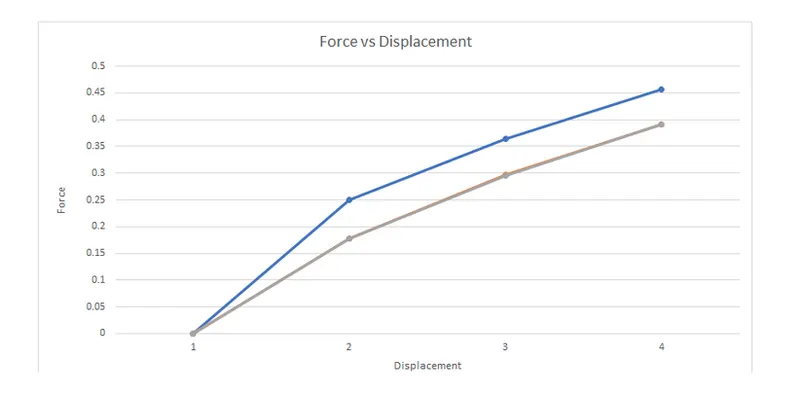
__________ Explicit Analysis

__________ Implicit Analysis

CONCLUSION:-

Explicit method is best suited for solving dynamic problems where rate of change of strain becomes important aspect such as an automotive crash, ballistic event, or even meteor impact whereas Implicit method

is very useful for static nonlinear problems where the events are much slower and the effects of strain rates are minimal.

Engineers choose between these two types of method for different applications based on-

• computational characteristics
• stability
• accuracy