LS-Dyna Explicit and Implicit Analysis Calculations
Objective: To perform explicit and implicit method calculations on a given equation with a tolerance value of 0.001.
Implicit method VS Explicit method
Explicit: As opposed to Implicit methods, the explicit method is a function of time. This scheme needs to consider as a function of time, velocity, acceleration, mass, and damping. Central Difference time integration (CDTI) is used to calculate field variables at respective nodal points in an explicit method. Since only a numerical solution is possible for a non-linear ordinary differential equation, this method is suited for non-linear problems. It requires the inversion of the lumped mass matrix instead of that of the global stiffness matrix in the implicit methods. In the CDTI, the equation of motion is evaluated at the previous time step (tn-1, where tn is the current timestep).
The explicit method or algorithm works in timestep increments, i.e., the displacements are calculated as the time proceeds. Consider the simulation of crash analysis. There is no deformation at timestep 1 (t=0 ms) since the impact is yet to occur. Gradually as time would progress the deformation also would change. Assume that at timestep 2, t is 5 ms, now the explicit algorithm will calculate the values of field variables when t=5 ms. This is how the solution proceeds. LS Dyna is one software based on explicit dynamics and is primarily used to solve problems such as Crash, Impact, Penetration, etc.
Implicit: In an implicit scheme, the displacement is not a function of time (i.e., x = constant). Hence, the velocities and accelerations, which are time derivatives of displacement, become zero, and the mass and damping factors can be neglected. The implicit method can be based on Newark’s method, Newton Raphson Method, etc. To solve a FEM problem using an implicit method, inversion of stiffness matrix (k) is required. Very Large deformation problems such as crash analysis can result in millions of degrees of freedom, effectively increasing the size of the stiffness matrix. Larger the stiffness matrix longer is the computational time required for its inversion. Hence there is a need for an explicit method that would prevent the inversion of the stiffness matrix. Implicit methods are mainly used in softwares such as Ansys, Nastran, Abaqus, etc.
|
|
Implicit method |
Explicit method |
|
Deformation |
small |
Large |
|
What causes large deformation |
Force and dynamic |
Velocity, acceleration with mass and inertia |
|
K matrix inversion |
yes |
No |
|
Time step size |
Large |
Small |
|
What limits the time step |
Accuracy |
Stability |
|
Cost per time step |
large |
Small |
|
What dominates the cost |
Matrix inversion |
Element process |
|
Parallel process |
Possible |
Not possible |
Explicit Analysis:
F(u)=`u^3+9u^2+4u`
Stiffness matrix K(u)=`(df)/(du`=`3u^2+18u+4`
Step 1:
u0=0.0
K(u0)=`3(0^2)+18(0)+4`
K(u0)=4
`DeltaF=1`
`Deltau1=(DeltaF)/(K(u0)`
`Deltau1=(1)/(4)`
`Deltau1=0.25`
`u1=u0+Deltau1`
`u1=0+0.25`
`u1=0.25`
Step 2:
K(u1)=`3(0.25^2)+18(0.25)+4`
K(u0)=8.6875
`DeltaF=1`
`Deltau2=(DeltaF)/(K(u1))`
`Deltau2=(1)/(8.6875)`
`Deltau2=0.1151`
`u2=u1+Deltau2`
`u2=0.25+0.1151`
`u2=0.3651`
Step 3:
K(u2)=`3(0.3651^2)+18(0.3651)+4`
K(u2)=10.971
`DeltaF=1`
`Deltau3=(DeltaF)/(K(u2))`
`Deltau3=(1)/(10.971)`
`Deltau3=0.09114`
`u3=u2+Deltau3`
`u3=0.3651+0.09114`
`u3=0.46`
Finally, To determine whether the analysis is in equilibrium,
`F(ext) = DeltaF+DeltaF+DeltaF`
`F(ext) = 1+1+1`
`F(ext) = 3`
f(int)=`underset(3)(u)^3+9underset(3)(u)^2+4underset(3)(u)`
f(int)=`0.46^3+9*0.46^2+4*0.46`
f(int)=3.841
F(ext) ≠ f(int), so they are not in equilibrium.
| Step i | `Delta`Fi | `Delta`ui | ui | F(ext)i | f(int)i | R=f(int)i-F(ext)i |
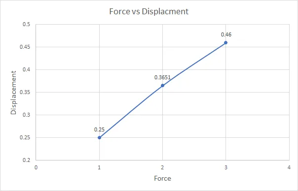
| 1 | 1 | 0.2500 | 0.25 | 1 | 1.578 | 0.578 |
| 2 | 1 | 0.1151 | 0.3651 | 2 | 2.708 | 0.708 |
| 3 | 1 | 0.09114 | 0.46 | 3 | 3.841 | 0.841 |
The graph between force and displacement for the explicit analysis:
Implicit Analysis:
F(u)=`u^3+9u^2+4u`
Stiffness matrix K(u)=`(df)/(du`=`3u^2+18u+4`
Step 1:
u0=0.0
K(u0)=`3(0^2)+18(0)+4`
K(u0)=4
`DeltaF=1`
`Deltau1=(DeltaF)/(K(u0)`
`Deltau1=(1)/(4)`
`Deltau1=0.25`
`u1=u0+Deltau1`
`u1=0+0.25`
`u1=0.25`
F(ext)=`DeltaF`=1
f(int)=`underset(1)(x)^3+9underset(1)(x)^2+4underset(1)(x)`
f(int)=`0.25^3+9*0.25^2+4*0.25`
f(int)=1.578125
`overset((0))(R)=`f(int)-F(ext)
`overset((0))(R)=1.578125-1`
`overset((0))(R)=0.578125`
`overset((0))(R)>10^-3`
Newton-Raphson iterations are necessary:
`underset(1)(u)=underset(1)(u)overset(0)`
`deltaoverset(1)(u)=-[Kunderset(1)overset(0)(u)]^-1*overset(0)(R)`
`deltaoverset(1)(u)=-[3(0.25^2)+18(0.25)+4]^-1*0.578125`
`deltaoverset(1)(u)=-0.066546`
`underset(1)(u)overset(1)()=underset(1)(u)overset(0)()+deltaoverset(1)(u)`
`underset(1)(u)overset(1)()=0.25-0.066546`
`underset(1)(u)overset(1)()=0.183454`
f(int)=`underset(1)(x)^3+9underset(1)(x)^2+4underset(1)(x)`
f(int)=`0.183454^3+9*0.183454^2+4*0.183454`
f(int)=1.042888
`overset((1))(R)=`f(int)-F(ext)
`overset((1))(R)=1.042888-1`
`overset((1))(R)=0.042888`
`overset((1))(R)>10^-3`
another Newton-Raphson iteration is necessary
`deltaoverset(2)(u)=deltaoverset(1)(u)-[Kunderset(1)overset(1)(u)]^-1*overset(1)(R)`
`deltaoverset(2)(u)=-0.066546-[3(0.183454)^2+18(0.183454)+4]^-1*0.042888`
`deltaoverset(2)(u)=-0.072339`
`underset(1)(u)overset(2)()=underset(1)(u)overset(0)()+deltaoverset(2)(u)`
`underset(1)(u)overset(2)()=0.25-0.072`
`underset(1)(u)overset(2)()=0.177661`
f(int)=`underset(1)(x)^3+9underset(1)(x)^2+4underset(1)(x)`
f(int)=`0.177661^3+9*0.177661^2+4*0.177661`
f(int)=1.000322
`overset((2))(R)=`f(int)-F(ext)
`overset((2))(R)=1.0003222-1`
`overset((2))(R)=0.000322`
`overset((2))(R)<10^-3`
Step 2:
u1=0.177661
K(u1)=`3(0.177661^2)+18(0.177661)+4`
K(u0)=7.292588
`DeltaF=1`
`Deltau2=(DeltaF)/(K(u0)`
`Deltau2=(1)/(7.292588)`
`Deltau2=0.137125`
`u2=u1+Deltau2`
`u2=0.177661+0.137125`
`u2=0.314786`
F(ext)=`DeltaF`=2
f(int)=`underset(2)(x)^3+9underset(2)(x)^2+4underset(2)(x)`
f(int)=`0.314786^3+9*0.314786^2+4*0.314786`
f(int)=2.182148
`overset((0))(R)=`f(int)-F(ext)
`overset((0))(R)=2.182148-2`
`overset((0))(R)=0.182148`
`overset((0))(R)>10^-3`
Newton-Raphson iterations are necessary:
`underset(2)(u)=underset(2)(u)overset(0)`
`deltaoverset(1)(u)=-[Kunderset(2)overset(0)(u)]^-1*overset(0)(R)`
`deltaoverset(1)(u)=-[3(0.314786^2)+18(0.31486)+4]^-1*0.182148`
`deltaoverset(1)(u)=-0.01828`
`underset(2)(u)overset(1)()=underset(2)(u)overset(0)()+deltaoverset(1)(u)`
`underset(2)(u)overset(1)()=0.314786-0.01828`
`underset(2)(u)overset(1)()=0.2965`
f(int)=`underset(2)(x)^3+9underset(2)(x)^2+4underset(2)(x)`
f(int)=`0.2965^3+9*0.2965^2+4*0.2965`
f(int)=2.00332
`overset((1))(R)=`f(int)-F(ext)
`overset((1))(R)=2.00332-2`
`overset((1))(R)=0.00332`
`overset((1))(R)>10^-3`
another Newton-Raphson iteration is necessary
`deltaoverset(2)(u)=deltaoverset(1)(u)-[Kunderset(2)overset(1)(u)]^-1*overset(1)(R)`
`deltaoverset(2)(u)=-0.01828-[3(0.2965)^2+18(0.2965)+4]^-1*0.00332`
`deltaoverset(2)(u)=-0.00035`
`underset(2)(u)overset(2)()=underset(2)(u)overset(1)()+deltaoverset(2)(u)`
`underset(2)(u)overset(2)()=0.2965-0.00035`
`underset(2)(u)overset(2)()=0.29616`
f(int)=`underset(2)(x)^3+9underset(2)(x)^2+4underset(2)(x)`
f(int)=`0.29616^3+9*0.29616^2+4*0.29616`
f(int)=2
`overset((2))(R)=`f(int)-F(ext)`
`overset((2))(R)=2-2`
`overset((2))(R)=0.0000`
`overset((2))(R)<10^-3`
Step 3:
u1=0.29616
K(u1)=`3(0.29616^2)+18(0.29616)+4`
K(u0)=9.59399
`DeltaF=1`
`Deltau3=(DeltaF)/(K(u0)`
`Deltau3=(1)/(9.59399)`
`Deltau3=0.10423`
`u3=u0+Deltau3`
`u3=0.29616+0.10423`
`u3=0.40039`
F(ext)=`DeltaF`=3
f(int)=`underset(1)(x)^3+9underset(1)(x)^2+4underset(1)(x)`
f(int)=`0.40039^3+9*0.40039^2+4*0.40039`
f(int)=3.10856`
`overset((0))(R)=`f(int)-F(ext)
`overset((0))(R)=3.10856-3`
`overset((0))(R)=0.10856`
`overset((0))(R)>10^-3`
Newton-Raphson iterations are necessary:
`underset(1)(u)=underset(1)(u)overset(0)`
`deltaoverset(1)(u)=-[Kunderset(1)overset(0)(u)]^-1*overset(0)(R)`
`deltaoverset(1)(u)=-[3(0.40039^2)+18(0.40039)+4]^-1*0.10856`
`deltaoverset(1)(u)=-0.00929`
`underset(3)(u)overset(1)()=underset(3)(u)overset(0)()+deltaoverset(1)(u)`
`underset(3)(u)overset(1)()=0.40039-0.00929`
`underset(3)(u)overset(1)()=0.39110`
f(int)=`underset(1)(x)^3+9underset(1)(x)^2+4underset(1)(x)`
f(int)=`0.39110^3+9*0.39110^2+4*0.39110`
f(int)=3.00088
`overset((2))(R)=`f(int)-F(ext`
`overset((2))(R)=3.00088-3`
`overset((2))(R)=0.00088`
`overset((2))(R)<10^-3`
| Step i | `Delta`Fi | `Delta`ui | ui | F(ext)i | f(int)i | R=f(int)i-F(ext)i |
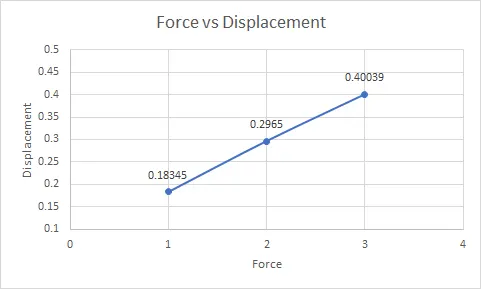
| 1 | 1 | 0.07234 | 0.18345 | 1 | 1.00032 | 0.00032 |
| 2 | 1 | 0.00035 | 0.2965 | 2 | 2 | 0 |
| 3 | 1 | 0.00929 | 0.40039 | 3 | 3.00088 | 0.00088 |
The graph between force and displacement for the implicit analysis:
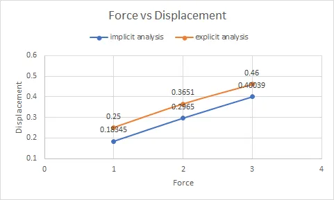
Comparison graph between the implicit analysis and explicit analysis:
Exact Calculations:
`F(u)= u^3+9u^2+4u = 1`
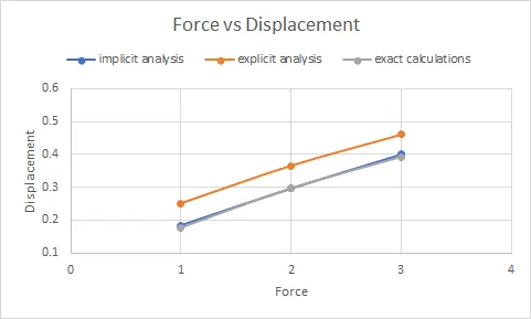
Upon calculation, we get u=0.1776
`F(u)= u^3+9u^2+4u = 2`
Upon calculation, we get u= 0.2962
`F(u)= u^3+9u^2+4u = 3`
Upon calculation, we get u= 0.3910
Comparison graph between implicit and explicit Force and exact calculations:
Conclusion:
The Implicit and Explicit calculations are carried out for a given equation. From the graphs, the Implicit method is more precise but time-consuming. It solemnly depends on element size and timestep, whereas explicit diverges somewhat from the exact result and needs more iterations to reach a good result.