Week - 2 - Explicit and Implicit Analysis

Challenge 2

Aim:
To solve the equation, F(u)= u3+9u2+4u, using Implicit and Explicit Methods.

Theory

Implicit Analysis

One method of solving for the unknowns {x} is through matrix inversion (or equivalent processes). This is known as an implicit analysis.

When the problem is nonlinear, the solution is obtained in several steps and the solution for the current step is based on the solution from the previous step. For large models, inverting the matrix is highly expensive and will require advanced iterative solvers (over standard direct solvers).

These solutions are unconditionally stable and facilitate larger time steps. Despite this advantage, the implicit methods can be extremely time-consuming when solving dynamic and nonlinear problems.

Explicit Analysis

Explicit analyses aim to solve for acceleration (or otherwise {x´´}). In most cases, the mass matrix is considered as “lumped” and thus a diagonal matrix.

Inversion of a diagonal matrix is straightforward and includes inversion of the terms on the diagonal only. Once the accelerations are calculated at the nth step, the velocity at the n+1/2 step and displacement at the n+1 step are calculated accordingly. In these calculations, the scheme is not unconditionally stable and thus smaller time steps are required. To be more precise, the time step in an explicit finite element analysis must be less than the Courant time step (i.e., the time taken by a sound wave to travel across an element)

Explicit vs Implicit Analysis

	Implicit	Explicit
Deformation	Small Deformation	Large Deformation
Causes of Deformation	Force and dynamic	Velocity, acceleration with mass and inertia
K matrix inversion	Yes	No
Time Step	Large	Small
What limits the time step	Accuracy	Stability
Cost per time step	Large	Small
Reason for cost	Matrix Inversion	Element Process
Parallel Process	Possible	Not Possible

Procedure

Explicit Analysis

• F(u)=u³+9u²+4u -1

Where, U is displacement,F is force and k is stiffness.
Incremental Displacements or Applied Force is represented using `Delta` U or `Delta`F respectively

• K(u)=F’(u)=3u²+18u+4 -2
• Take , u=0 in 2
• K(u=0)=3*0² + 18*0 +4 =4
• `Delta` F=K*`Delta` U -3
• Taking `Delta` F=1, we get
• 1=K*`Delta` U₁
  1=4* `Delta` U₁
• = `Delta` U₁ = ¼=0.25
• U₁ = U₀+ `Delta` U₁
  = U₁=0 + 0.25 =0.25
  U₁ =0.25
  F_int =F(U₁)=0.25³ + 9*0.25² + 4 * 0.25
• =F_int =1.578

Take U₁=0.25 in 2
K(U₁)=3*0.25²+18*0.25+4=8.6875.

From 3,
`Delta` U₂=1/8.6875 =0.1151

U₂=U₁+`Delta` U₂=0.25+0.1151 =0.3651

Substitute U₂ in 1

F_int= 0.3651³+9*0.3651²+4*0.3651 =2.708

Take U₂=0.3651 in 2
K(U₂)=3*0.3651²+18*0.3651+4=10.9716
From 3,
`Delta` U₃=1/10.9716 =0.09114

U₃=U₂+`Delta` U₃
=0.3651+0.09114=0.46

Subsitute U₃ in 1
F_int=0.46³+9*0.46²+4*0.46 =3.841

F_ext=3
F_ext=/=F_int, therefore the system is not in equilibrium

Step i	`Delta`Fi	`Delta`Ui	Ui	Fext	Fint	R=Fext-Fint
1	1	0.25	0.25	1	1.578	0.578
2	1	0.1151	0.3651	2	2.708	0.708
3	1	0.09114	0.46	3	3.841	0.841

Implicit Analysis

• We will be using a Tolerance of 0.01 for the Newton-Raphson Iteration
• F(u)=u³+9u²+4u -1

Where, U is displacement,F is force and k is stiffness.
Incremental Displacements or Applied Force is represented using `Delta` U or `Delta` F respectively

• K(u)=F’(u)=3u²+18u+4 -2
• Take , u=0 in 2
• K(u=0)=3*0² + 18*0 +4 =4

`Delta` F=K*`Delta` U

Taking `Delta` F=1, we get

1=K*`Delta` U₁
1=4* `Delta` U₁

= `Delta` U₁ = ¼=0.25

U₁ = U₀+ `Delta` U₁
= U₁=0 + 0.25 =0.25
U₁ =0.25
F_int =F(U₁)=0.25³ + 9*0.25² + 4 * 0.25

=F_int =1.578

R₀=F_int – F_ext=1.578 – 1 =0.578
This is greater than our tolerance of 10^-2, so Newton-Raphson correction is needed.

Correction is U₁=U₁ ⁽¹⁾

`Delta`U^j+1 = −[k(u^j)]⁻¹*R_j
On substituting j=0,

`Delta` U(1)= -[k(u₁(0)]^-1 * R₀

`Delta` U(1)= - [(3*0.25²+18*0.25+4)^-1*0.578

`Delta` U(1)=-0.0665

U₁ = U₁(0)+ Delta U(1)

U₁ = 0.25-0.0665

U₁=0.1835

Residual R₁=F_int – F_{ext -3}
F_int =F(U₁)=0.1835³ + 9*0.1835² + 4 * 0.1835
F_int=1.0432
R₁=1.0432 -1 =0.0432, substituting F_int F_ext in 3

R₁ is greater than our tolerance of 10^-2, so another iteration is needed.

`Delta`U(2) = `Delta`U(1) − [k(u(1)¹)]⁻¹R(1)
`Delta` U(2)=-0.0665 – [(3*0.1835² +9*0.1835+4)^-1*0.0432]

`Delta` U(2)= -0.0714

U₁ = 0.25-0.0714

U₂=0.1786

Residual R₀=F_int – F_ext
F_int =F(U₁)=0.1786³ + 9*0.1786² + 4 * 0.1786
F_int=1.0071

R₀=1.0071-1 =0.0071 which is lower than our tolerance of 10^-2. Therefore, no further iterations are needed.

U₁=0.1786.

Similarly, we derive U₂=0.2966 and U₃=0.3911

Step i	`Delta`Fi	`Delta`Ui	Ui	Fext	Fint	R=Fext-Fint
1	1	0.25	0.1786	1	1.0071	0.0071
2	1	0.1374	0.2966	2	2.0042	0.0042
3	1	0.1041	0.3911	3	3.008	0.008

Comparison

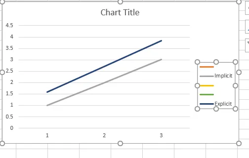
It can be observed that in Explicit Analysis, the solution drifts from the exact value, indicating a lack of equilibrium in the external and internal forces.

However, in the case of Implicit Analysis, the Residual Force is negligible and is close to the exact value. That is, the solution derived from implicit Analysis is more accurate. This is because we used Newton-Raphson Iterations to enable equilibrium between internal and external Forces.

Conclusion

A nonlinear analysis is illustrated using an incremental explicit and implicit procedure.

The results are plotted for comparison. It is evident from the results that the explicit analysis drifts from the true solution.

In Implicit Analysis, which includes Newton-Raphson iterations to enforce equilibrium between internal and external forces, the results are significantly more accurate to the true solution.