Week - 2 - Explicit and Implicit Analysis

AIM: To solve the given equation by Explicit and Implicit method. 

ANSWER 1:

• Final Element Method (FEM) is a numerical method to solve the partial differential equations. And those differential equations can be solve by two methods.

1. EXPLICIT METHOD    2. IMPLICIT METHOD

Explicit Method: 

• LS-DYNA primarily used for solving non linear transient dynamic problems using explicit FEM.
• So considering time step , the time step in explicit method is very fast but the method only works when when step delta-t is small.
• Explicit method is a time dependant.
• Explicit method generally used to calculate given system of different time step with current time step.
• It can be used when the process is fast.
• It is a conditionally stable method.

IMPLICIT Method:

• LS-DYNA has capability to solve implicit method too.
• It is a time independant function. 
• It is generally used to solve the static problems.
• The implicit method finds a solution by solving an equation that includes both the current and later states of the given system..
• The computation time for this method is more than the expliciti method.
• It can be use in the slower process. 

F(u) = u3+9u2+4u use this equation and solve using both Explicit and Implicit Methods ( have a tolerence of 0.001).

For this example three equal load increments (or steps) of ∆F = 1 unit each are used to load the tension bar.Use is made of the relationship ΔF=kΔu">ΔF=kΔu. The analysis proceeds as follows.

By Explicit Method:

`f(u)=u^3+9u^2+4u`

`:. k(u)=(df)/(du)=3u^2+18u+4`

STEP 1 :

put  `u0=0,0` then `k(u0)=4`

`DeltaF=1`

Now,  `Deltau1=(DeltaF)/(k(u0))=1/4=0.25`

`u1=u0+Deltau1=0+.25=0.25`

STEP 2:

`k(u1)=3(u1)^2+18(u1)+4`

`:. k(u1)=3*(0.25)^2+18*0.25+4`

`k(u1)=8.69`

`DeltaF=1`

`Now, Delta(u2)=(DeltaF)/(k(u1))=1/8.69=0.12`

`u2= u1+Deltau2=0.25+0.12=0.37`

STEP 3 

`k(u2)=3(u2)^2+18(u2)+4`

`:. k(u2)=3*(0.37)^2+18*0.37+4=11.07`

`DeltaF=1`

`Now, Delta(u3)=(DeltaF)/(k(u2))=1/11.07=0.09`

`u3= u2+Deltau3=0.37+0.09=0.46`

Finally, from the three steps the following results are obtained.
`Fext = ∆F + ∆F + ∆F = 3.0`

(Fint)1=`(u1)^3+9(u1)^2+4(u1)=0.25^3+9*0.25^2+4*0.25=1.58`

(Fint)2=`(u2)^3+9(u2)^2+4(u2)=0.37^3+9*0.37^2+4*0.37=2.8`

(Fint)3= `(u3)^3+9(u3)^2+4(u3)=0.46^3+9*0.46^2+4*0.46=3.84`

It is evident from the results that external and internal forces are NOT in equilibrium because
Fext `!=` fint.

SUMMARY:

Step i	`DeltaFi`	`Deltaui`	`ui`	(Fext)i	(fint)i	fint-Fext=R
1	1.0	0.25	0.25	1	1.58	0.58
2	1.0	0.12	0.37	2	2.8	0.8
3	1.0	0.09	0.46	3	3.84	0.84

By Implicit Method:

`f(u)=u^3+9u^2+4u`

`:. k(u)=(df)/(du)=3u^2+18u+4`

STEP 1:

put  `u0=0,0` then `k(u0)=4`

`DeltaF=1`

Now,  `Deltau1=(DeltaF)/(k(u0))=1/4=0.25`

`u1=u0+Deltau1=0+.25=0.25`

 Check the residual,

`Fext=DeltaF=1`

Fint= `(u1)^3+9(u1)^2+4(u1)=0.25^3+9*0.25^2+4*0.25=1.58`

`R^(0)=fInt-Fext=1.58-1=0.58`

`||R^(0)|| > 10^(−2)` so Newton-Raphson iterations are necessary.

Calculate correction to 

`u1=u1^(0)`

`deltau^1=-[k(u1^(0))]^-1R^0= -1/8.69*0.58=-0.067`

the updated value: 

`u1^(0)+deltau^(1)=0.25-0.067=0.183`

Check the residual again,

`Fext=DeltaF=1`

Fint= `(u1^1)^3+9(u1^1)^2+4(u1^1)=1.04`

`R^1=fInt-Fext=0.039`

`||R^1||>10^(-2)`  

So another interation is required.

Calculate the new total correction to `u1 = u1^(0)`

`deltau^((2))=deltau^((1))-[k(u)^((1))]^-1R^((1))`

`=-0.067-8.69^-1-0.03`

`deltau^((2))=-0.0714`

The updated value of ,  `u1^((2))=u1^((0))=delta^((2))`

`=0.25-0.0714=0.1786`

Check the residual ;  

`Fext=1 and FInt=(u1)^3+9(u1)^2+4(u1)`

`=0.1786^3+9*0.1786^2+4*0.1786=1.0071`

`R^((2))=fInt-Fext=1.0071-1=0.0071`

`||R^((2))||<10^-2`

`:.` No iteration is needed , `u1=0.1786`

Step 2 & 3 : We will calculate this as above 

and we got `u2=0.2966 and u3=0.3911`

Step i	`DeltaFi`	`ui`	(Fext)i	`(FInt)i`	`fInt-Fext=R`
1	1	0.1786	1	1.007	0.007
2	1	0.2965	2	2.004	0.004
3	1	0.3911	3	3.001	0.001

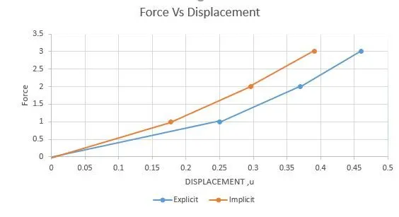
Force Vs Displacement

CONCLUSION:

• The Explicit and Implicit function solve as per the steps showed in pdf.
• The force vs displacement graph is plotted.