Week - 2 - Explicit and Implicit Analysis
AIM:
Solve the given equation,F(u)=u3+9u2+4u in both implici and explicit method.
OBJECTIVE:
- Solve the equation, F(u)=u3+9u2+4u using explicit method
- Solve the equation,F(u)=u3+9u2+4u using implicit method.
1) Brief intro on EXPLICIT METHOD.
Explicit methods calculate the state of a system at a later time from the state of the system at the current time, while implicit methods find a solution by solving an equation involving both the current state of the system and the later one.
In an explicit numerical method S would be evaluated in terms of known quantities at the previous time step n. ... Usually a matrix or iterative solution must be used to compute the new quantities. Numerical stability has to do with the behavior of the solution as the time-step dt is increased.
In explicit analysis ,solution is performed with direct iterative calculation.however,error accumulate and the answer will diverge over a time from answer you are model but the method is fast and inexpensive computationally.
CALCULATION:
To perform a Non-linear static analysis on a bar element constrained on one side while subjected to an external load on the other end using an Incremental load scheme using both Implicit and Explicit method and then solve them numerically.
Let us consider a bar element constrained on all DOFs on one side whereas the opposite side is un-constrained. Consider a force acting on the bar in the axial direction causing Tension in the bar.
The internal force f(u) experienced on the bar is a non-linear (higher-order) function of displacement.
f(u)=u3+9u2+4
NUMERICAL SOLUTION:
Given, Internal force,
f(u)=u3+9u2+4u -----(1)
We can compute the stiffness from the above equation as,
k=df/du=3u2+18u+4 -----(2)
we know that ∆F=k×∆u -----(3)
Where, F -> External load, ΔF-> Load Increment
f(u) -> Internal force, k -> Stiffness
u -> Displacement , Δu -> Displacement Increment
Step 1: At first load step, ΔF = 1, u0 = 0From (2), k(u0)=3(0)+18(0)+4=4
From (3), ∆u1=∆F/k=1/4=0.25
Therefore, u1=u0+∆u1
Where, u0 -> Initial displacement at no load
u1 -> Final displacement after 1st step load
Δu1 -> Change in displacement caused due to step load, ΔF=1
u1=0+0.25=0.25
u1=0.25
Step 2: At second load step, ΔF = 1, u1 = 0.25From (2), k(u1)=3(0.25)2+18(0.25)+4=8.687
From (3), ∆u2=∆F/(k(u1))=1/8.687=0.115
Therefore, u2=u1+∆u2u1=0.25+0.115=0.365
u2=0.365
Step 3: At third load step, ΔF = 1, u1 = 0.25From (2), k(u2)=3(0.365)2+18(0.365)+4=10.97
From (3), ∆u3=∆F/(k(u2))=1/10.97=0.091
Therefore, u3=u2+∆u3u1=0.365+0.091=0.456
u3=0.456
Hence the result that we obtain from the implicit analysis are,
F+ΔF+ΔF=1+1+1
F=3
Internal force,f=f(u3)=f(0.456)
f(u3)=〖(0.456)〗3+9×〖(0.456)〗2+4×(0.456)
f(u3)=3.79
Therefore, F≠f i.e External force ≠ Internal force
Hence, the system is not in equilibrium.
TABLE FOR EXPLICIT:
| STEP | F | u1 | F(external) | F(internal) | R=f-F |
| 1 | 1 | 0.25 | 1 | 1.578 | 0.578 |
| 2 | 1 | 0.365 | 2 | 2.707 | 0.707 |
| 3 | 1 | 0.456 | 3 | 3.79 | 0.79 |
BREIF INTRO OF IMPLICIT METHOD:
In the implicit method, we implement the “Incremental Explicit Load Scheme” where three equal steps of load increment of ΔF = 1 are used to load the bar in tension. However, unlike the explicit method, here we perform a Newton-Raphson iteration at the end of each time step to minimize the Residue and enforce equilibrium at the system before proceeding to the next load step.
wkt, Residue, R(u)=f−F
Upon expanding the above equation as a Taylor series, we get,
Rj+1=Rj(uj)+dR(uj)du〖δu〗j+1+⋯
Hence ignoring higher-order terms, we get,
Rj+1=Rj(uj)+dR(uj)du〖δu〗j+1=Rj+k(uj)〖δu〗j+1
To attain equilibrium, R(j+1)=0
Hence solving for 〖δu〗(j+1), we get
〖δu〗j+1=〖-[K(uj)]〗-1×Rj
In this Implicit method, we need to reduce the Residue below a tolerance level, because we cannot eliminate the residue completely using few Newton-Raphson iterations done numerically.
Step 1: At first load step, ΔF = 1, u0 = 0From (2),
k(u0)=3(0)+18(0)+4=4
From (3), ∆u1=∆F/k=1/4=0.25
Therefore,u1=u0+∆u1u1=0+0.25=0.25
Internal force f(u1)=〖(0.25)〗3+9×〖(0.25)〗2+4×(0.25)=1.578
Check Residue: R(u)=f−F=1.578−1=0.578
R(0)>10-2 -> Perform Newton-Raphson Iteration
Newton-RaphsonIteration 1: u1= u1(0)=0.25
〖δu〗(1)=〖-[K(uj)]〗-1×Rj
〖δu〗(1)=〖-[8.68]〗-1×0.578=-0.0665
〖δ〗〖u1〗(1)=〖u1〗(0)+〖δu〗(1)=0.25+(-0.0665)=0.1835
f(〖u1〗(1))=1.0432
Check Residue: R(u)=f-F=1.0432-1=0.0432
R(1)>10-2 -> Perform Newton-Raphson Iteration
Similarly, as we perform two more Iterations we will reach at a value with residue less than 0.01
u1=〖u1〗(3)=0.17764
Step 2: At second load step, ΔF = 1, u1 = 0.17764
From (2), k(u1)=3(0.17764)+18(0.17764)+4=7.28
From (3), ∆u2=∆F/k=1/7.28=0.13736
Therefore,u2=u1+∆u2u2=0.177+0.13736=0.31436
Internal force (u2)=〖(0.31)〗3+9×〖(0.31)〗2+4×(0.31)=2.1779
Check Residue: R(u)=f−F=2.1779−2=0.1779
R(0)>10-2
Like before perform Newton-Raphson iterations to minimize the residue.
This would result in,
u2=0.29649
Similarly, if you apply the third load increment and after performing successively the Newton-Raphson iteration, we get,
u3=0.39111
Hence the result that we obtain from the implicit analysis .
TABLE FOR IMPLICIT :
| STEPS | ∆F1 | U1 | F(external) | F(internal) | R=f-F |
| 1 | 1 | 0.17764 | 1 | 1.0002 | 0.0002 |
| 2 | 1 | 0.29649 | 2 | 2.0032 | 0.0032 |
| 3 | 1 | 0.39111 | 3 | 3.0009 | 0.0009 |
PLOT GRAPH:
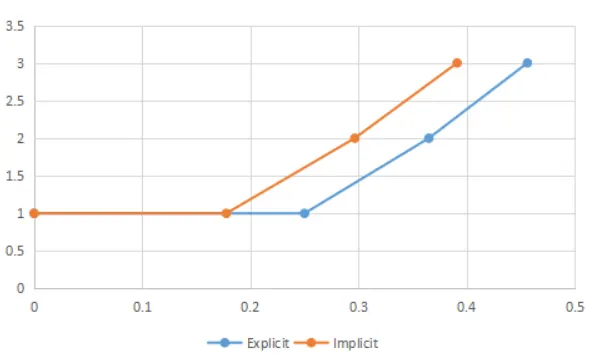
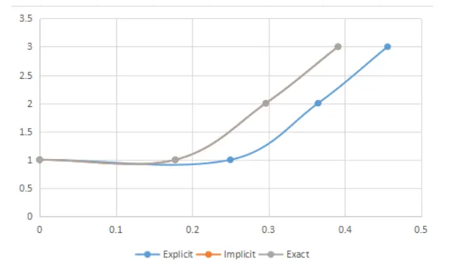
The graph shows the value of force verses displacement by both implicit and explicit method
(i) Comparison of force vs Displacement of implicit and explicit method.
(ii) Comparsion of force vs displacement of explicit,implicir,exact solution method
RESULT AND CONCLUSION:
The result are plotted for comparsion. It proof from the result that the explicit analysis drifts more than an implicit analysis used,which includes newton-raphson iteration to enforce equlibrium between external and internal forces.