Week 2 Air standard Cycle

About the Otto Cycle:

The Otto cycle is a theoretical thermodynamic cycle that describes the operation of a typical spark-ignition piston engine, such as those used in most gasoline-powered vehicles. It consists of four main processes: intake, compression, power, and exhaust. Here's a step-by-step explanation of each process:

1. Intake (Process 1-2):

- The intake valve opens, allowing the air-fuel mixture (usually gasoline and air) to enter the cylinder from the intake manifold.

- As the piston moves downward during the intake stroke, the volume inside the cylinder increases, drawing in the air-fuel mixture.

- The intake stroke ends when the intake valve closes, trapping the air-fuel mixture inside the cylinder.

2. Compression (Process 2-3):

- With both the intake and exhaust valves closed, the piston moves upward during the compression stroke, compressing the air-fuel mixture.

- As the volume decreases, the pressure and temperature of the mixture increase significantly.

- This compression raises the mixture's energy content and prepares it for efficient combustion.

3. Power (Process 3-4):

- When the piston reaches the top of its stroke (top dead center), the spark plug ignites the compressed air-fuel mixture.

- The ignited mixture undergoes rapid combustion, releasing heat energy.

- This sudden increase in pressure forces the piston downward, creating mechanical work on the crankshaft.

- The power stroke is where the engine produces its useful work, which ultimately propels the vehicle.

4. Exhaust (Process 4-1):

- After the power stroke, the exhaust valve opens, and the piston moves upward during the exhaust stroke.

- This upward movement pushes the burned gases out of the cylinder and into the exhaust manifold.

- The cycle completes when the piston reaches the top again, and the exhaust valve closes, ready to start a new cycle.

The Otto cycle is an idealized representation, and in real engines, there are variations due to factors like friction, heat losses, and incomplete combustion. However, it provides a fundamental understanding of how internal combustion engines operate.

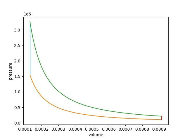
Below down we have conisdered the engine kinematics to get the ideal otto cycle pressure-volume plot, In terms of clearance volume following expression is being used :

inputs for specific output have been considered as follows:

bore=0.1

stroke=0.1

con_rod=0.15 (connecting rod length)

cr=7 (compression ratio)

p1=101325 pa (initial pressure)

t1=500 (initial temperature)

gamma=1.4

t3=2300 (termperature during power stroke)

crank angle may vary in between 0 to 180 depending on the position of crank.

here we have calculated for 50 values of crank angles to get volumes.

import math
import matplotlib.pyplot as plt 

def engine_kinematics(bore,stroke,con_rod,start_crank,end_crank):

	#geometric parameters

	a=stroke/2
	R=con_rod/a

	#Volume Parameters
	V_s=math.pi*(1/4)*pow(bore,2)*stroke
	V_c=V_s/(cr-1)

	sc=math.radians(start_crank)
	ec=math.radians(end_crank)

	num_values=50

	d_thetha= (ec-sc)/(num_values-1)

	V=[]
	for i in range (0,num_values):
		thetha=sc+i*d_thetha

		term1=0.5*(cr-1)
		term2=R+1-math.cos(thetha)
		term3= pow(R,2)-pow(math.sin(thetha),2)
		term3=pow(term3,0.5)

		V.append((1+term1*(term2-term3))*V_c)

	return V


 #inputs
p1=101325
t1=500
gamma=1.4
t3=2300

#geometric parameters
bore=0.1
stroke=0.1
con_rod=0.15
cr=7

#volume computations
v_s=(math.pi/4)*pow(bore,2)*stroke
v_c=v_s/(cr-1)
v1=v_c+v_s

#state point 2
v2=v_c

#p2v2^gamma=p1v1^gamma
p2=p1*pow(v1,gamma)/pow(v2,gamma)

#p2v2/t2=p1v1/t1| rhs=p1v1/t1 | p2v2/t2=rhs | t2=p2v2/rhs
rhs=p1*v1/t1
t2=p2*v2/rhs
V_compression= engine_kinematics(bore, stroke,con_rod, 180,0)

constant=p1*pow(v1,gamma)

P_compression=[]
for v in V_compression:
 	P_compression.append(constant/pow(v,gamma))

#state point 3
v3=v2

#p3v3/t3=p2v2/t2 |rhs=p2v2/t2 |p3=rhs*t3/v3

rhs=p2*v2/t2
p3=rhs*t3/v3
V_expansion= engine_kinematics(bore, stroke,con_rod, 0,180)

constant=p3*pow(v3,gamma)

P_expansion=[]
for v in V_expansion:
 	P_expansion.append(constant/pow(v,gamma))


#state point 4
v4=v1

#p4v4^gamma =p3v3^gamma

p4=p3*pow(v3,gamma)/pow(v4,gamma)

#p4v4/t4=rhs
t4=p4*v4/rhs

thermal_efficinecy= 1-(1/pow(cr,(gamma-1)))
print(thermal_efficinecy)

plt.plot([v2,v3],[p2,p3])
plt.plot(V_compression,P_compression)
plt.plot(V_expansion,P_expansion)
plt.plot([v4,v1],[p4,p1])
plt.xlabel('volume')
plt.ylabel('pressure')
plt.show()

P-V Diagram

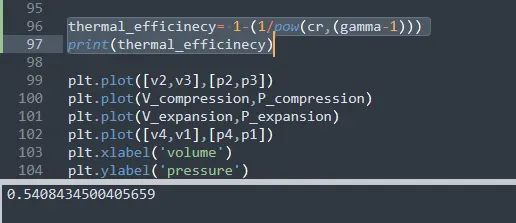
Thermal Efficiency = 0.5408

For any further verification kindly check the zip file contaning the pythone code file and output image file.