Week 2 Air standard Cycle
Based on the concepts you have learnt during the forward kinematics routine, go
ahead and write code that can solve an Otto cycle and make plots for it.
Here are the requirements
1. Your code should create a pressure-volume (PV) diagram
2. You should output the thermal efficiency of the engine.
Aim:
To develop a code that can solve an Otto Cycle, plot the PV diagram and derive the thermal efficiency of the engine.
Objective:
Using the forward kinematics procedure, develop a program to solve an Otto cycle and generate related charts. The program should generate a pressure-volume (PV) diagram and determine the engine's thermal efficiency.
Problem Statement:
A simplified framework for comprehending the operation of spark-ignition internal combustion engines, which are frequently used in gasoline-powered cars, is provided by the air standard Otto cycle depicted in Figure 3. This cycle is an idealized thermodynamic cycle.
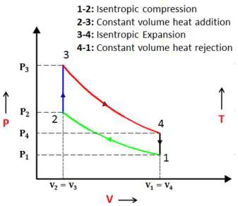
Figure 3: PV diagram of air standard Otto cycle.
Although idealized, the Otto cycle provides useful insights into the thermodynamic processes that drive engine performance. The cycle's four major strokes (intake, compression, combustion, and expansion) provide a theoretical basis for study, but real-world engines may differ due to heat transmission, friction, and combustion complexities. The primary stage in the cycle are as follows:
-
Intake: The cycle starts with the intake stroke, where a mixture of air and fuel is drawn into the engine cylinder. This intake stage is often modeled as an isentropic compression, characterized by a rise in pressure and temperature due to the piston's motion.
-
Compression: Subsequent to intake, the compression stroke involves adiabatic and reversible compression of the air-fuel mixture. This process raises pressure and temperature, readying the mixture for combustion.
-
Combustion: During combustion, which occurs at constant volume, the compressed mixture ignites via a spark plug. This rapid combustion heightens temperature and pressure, leading to piston movement and energy conversion.
-
Expansion: Following combustion, the expansion stroke ensues, where hot gases undergo adiabatic and reversible expansion, propelling the piston upwards. This phase decreases pressure and temperature while extracting mechanical work from the engine.
The Otto cycle simplifies the complexities of internal combustion engines, making it a valuable tool for research. It serves as a reliable benchmark for assessing engine efficiency, power production, and thermal behavior. Throughout the cycle, engineers and researchers study operating and design characteristics to advance internal combustion engines and automotive technologies.
The governing equations for an Otto cycle are:
Swept Volume in m3:
`V_s = pi/4 ast d^2 ast L`
Clearance Volume in m3:
`V_c = V_s / (r - 1)`
Volume at Stage 1 (BDC) in m3:
`V_1 = V_4 = V_s + V_c`
Volume at Stage 2 (TDC) in m3:
`V_2 = V_3 = V_c`
Relation between Pressure (MPa) and Volume (m3):
`P_1 ast V_1^gamma = P_2 ast V_2^gamma`
Ideal Gas Equation of State:
`(P_1 ast V_1) / T_1 = (P_2 ast V_2) / T_2`
Instantaneous Volume (m3):
`V_theta = V_c + (1+(r-1)/2) ast {1+R-cos theta - (R^2 - sin^2theta)^frac{1}{2}}`
Instantaneous Pressure (MPa):
`P_theta ast V_theta^gamma = P_2 ast V_2^gamma`
Thermal Efficiency:
`eta = 1 - 1/r^(gamma-1)`
Where,
𝒅 is the bore diameter; 𝑳 is the stroke; 𝑳𝒄𝒓 is the connecting rod length; 𝒓 is the compression ratio; 𝜸 is the specific heat ratio; 𝜽 is the crank angle
Program:
"""
Author: Aksharat Jain
"""

import math
import matplotlib.pyplot as plt

def engine_kinematics(bore, stroke, con_rod, cr, start_crank, end_crank):
    # Geometric Parameters
    a = stroke / 2
    R = con_rod / a

    # Volume Parameters
    v_s = math.pi * (1 / 4) * pow(bore, 2) * stroke   # Swept Volume
    v_c = v_s / (cr - 1)                              # Clearance volume

    sc = math.radians(start_crank)   # Starting crank angle
    ec = math.radians(end_crank)     # Ending crank angle

    num_values = 40

    dtheta = (ec - sc) / (num_values - 1)   # Crank angle spacing

    V = []

    for i in range(0, num_values):
        theta = sc + i * dtheta

        term1 = 0.5 * (cr - 1)
        term2 = R + 1 - math.cos(theta)
        term3 = pow(R, 2) - pow(math.sin(theta), 2)
        term3 = pow(term3, 0.5)

        V.append((1 + term1 * (term2 - term3)) * v_c)

    return V

def otto_cycle(bore, stroke, con_rod, cr, start_crank, end_crank):
    # Inputs
    p1 = 101325
    t1 = 500
    gamma = 1.4
    t3 = 2300

    # Volume computation
    v_s = math.pi * (1 / 4) * pow(bore, 2) * stroke
    v_c = v_s / (cr - 1)
    v1 = v_s + v_c

    # State point 2
    v2 = v_c

    # P2 V2^gamma = P1 V1^gamma
    p2 = p1 * (pow(v1, gamma) / pow(v2, gamma))

    # P2 V2/T2 = P1 V1/T1 | RHS = P1 V1/T1 | P2 V2/T2 = RHS | T2 = P2 V2/RHS
    rhs = (p1 * v1) / t1
    t2 = (p2 * v2) / rhs

    V_compression = engine_kinematics(bore, stroke, con_rod, cr, start_crank, end_crank)

    constant = p1 * pow(v1, gamma)

    P_compression = []

    for v in V_compression:
        P_compression.append(constant / pow(v, gamma))

    # State point 3
    v3 = v2

    # P3 V3/T3 = P2 V2/T2 | RHS = P2 V2/T2 | P3 V3/T3 = RHS | P3 = RHS * T3/V3
    rhs = (p2 * v2) / t2
    p3 = rhs * (t3 / v3)

    V_expansion = engine_kinematics(bore, stroke, con_rod, cr, end_crank, start_crank)

    constant = p3 * pow(v3, gamma)

    P_expansion = []

    for v in V_expansion:
        P_expansion.append(constant / pow(v, gamma))

    # State point 4
    v4 = v1

    # P4 V4^gamma = P3 V3^gamma
    p4 = (p3 * (pow(v3, gamma)) / (pow(v4, gamma)))

    # P4 V4/T4 = RHS
    t4 = (p4 * v4) / rhs

    return V_compression, P_compression, V_expansion, P_expansion, v1, p1, v2, p2, v3, p3, v4, p4

def plot_pv_diagram(V_compression, P_compression, V_expansion, P_expansion, v1, p1, v2, p2, v3, p3, v4, p4):
    plt.plot([v2, v3], [p2, p3], label="Isochoric Heat Addition")
    plt.plot(V_compression, P_compression, label="Compression")
    plt.plot(V_expansion, P_expansion, label="Expansion")
    plt.plot([v4, v1], [p4, p1], label="Isochoric Heat Rejection")
    plt.xlabel('Volume (m^3)')
    plt.ylabel('Pressure (Pa)')
    plt.title('Otto Cycle PV Diagram')
    plt.grid(True)
    plt.legend()
    plt.show()

# Geometric Parameters
bore = 0.1
stroke = 0.1
con_rod = 0.15
cr = 7
start_crank = 180
end_crank = 0

V_compression, P_compression, V_expansion, P_expansion, v1, p1, v2, p2, v3, p3, v4, p4 = otto_cycle(bore, stroke, con_rod, cr, start_crank, end_crank)
plot_pv_diagram(V_compression, P_compression, V_expansion, P_expansion, v1, p1, v2, p2, v3, p3, v4, p4)

# Calculating thermal efficiency of the Otto Cycle
def thermal_efficiency(cr):
    gamma = 1.4  # Specific heat ratio for air

    efficiency = 1 - (1 / (cr ** (gamma - 1)))
    return (efficiency*100)

# Assuming you have calculated cr in your otto_cycle function
cr = 7  # Compression ratio

efficiency = thermal_efficiency(cr)
print("\n Thermal Efficiency:", efficiency)
Explanation:
The code provided implements simulations for the Otto cycle, a fundamental thermodynamic cycle representing the idealized operation of a spark-ignition internal combustion engine. Additionally, it calculates the thermal efficiency of the Otto cycle, which is a crucial parameter for assessing the performance of such engines.
Importing Libraries:
import math
import matplotlib.pyplot as plt-
math: Utilized for various mathematical computations such as trigonometric functions and exponentiation.
-
matplotlib.pyplot: Employed for generating graphical visualizations, particularly for plotting pressure-volume (PV) diagrams.
'engine_kinematics' Function:
def engine_kinematics(bore, stroke, con_rod, cr, start_crank, end_crank):
    # Geometric Parameters
    a = stroke / 2
    R = con_rod / a

    # Volume Parameters
    v_s = math.pi * (1 / 4) * pow(bore, 2) * stroke   # Swept Volume
    v_c = v_s / (cr - 1)                              # Clearance volume

    sc = math.radians(start_crank)   # Starting crank angle
    ec = math.radians(end_crank)     # Ending crank angle

    num_values = 40

    dtheta = (ec - sc) / (num_values - 1)   # Crank angle spacing

    V = []

    for i in range(0, num_values):
        theta = sc + i * dtheta

        term1 = 0.5 * (cr - 1)
        term2 = R + 1 - math.cos(theta)
        term3 = pow(R, 2) - pow(math.sin(theta), 2)
        term3 = pow(term3, 0.5)

        V.append((1 + term1 * (term2 - term3)) * v_c)

    return V
This function calculates the engine kinematics, focusing on determining volumes at different crank angles. It involves several steps:
-
Geometric Parameters: Calculates key geometric parameters such as crank radius, stroke, and clearance volume.
-
Volume Parameters: Computes the swept volume and clearance volume based on bore, stroke, and compression ratio.
-
Crank Angle Spacing: Determines the spacing between crank angles for calculation precision.
-
Volume Calculation Loop: Iterates through crank angles to compute corresponding volumes using the kinematic equations.
'otto_cycle' Function:
def otto_cycle(bore, stroke, con_rod, cr, start_crank, end_crank):
    # Inputs
    p1 = 101325
    t1 = 500
    gamma = 1.4
    t3 = 2300

    # Volume computation
    v_s = math.pi * (1 / 4) * pow(bore, 2) * stroke
    v_c = v_s / (cr - 1)
    v1 = v_s + v_c

    # State point 2
    v2 = v_c

    # Calculations for compression process
    ...

    # State point 3
    v3 = v2

    # Calculations for expansion process
    ...

    # State point 4
    v4 = v1

    # P4 V4^gamma = P3 V3^gamma
    p4 = (p3 * (pow(v3, gamma)) / (pow(v4, gamma)))

    # P4 V4/T4 = RHS
    t4 = (p4 * v4) / rhs

    return V_compression, P_compression, V_expansion, P_expansion, v1, p1, v2, p2, v3, p3, v4, p4
The 'otto_cycle' function is responsible for simulating the entire Otto cycle. The steps involved are:
-
Input Parameters: Defines initial parameters such as initial pressure, initial temperature, specific heat ratio (gamma), and temperature at state 3.
-
Volume Computation: Calculates the volumes corresponding to different states of the cycle.
-
Compression Process: Computes pressures during the compression process from state 1 to state 2.
-
Expansion Process: Calculates pressures during the expansion process from state 3 to state 4.
-
State Points 4 and 5: Determines the final state points based on volume and pressure relationships.
-
Isochoric Heat Rejection: Computes pressure during the isochoric heat rejection process from state 4 to state 1.
'plot_pv_diagram' Function:
def plot_pv_diagram(V_compression, P_compression, V_expansion, P_expansion, v1, p1, v2, p2, v3, p3, v4, p4):
    plt.plot([v2, v3], [p2, p3], label="Isochoric Heat Addition")
    plt.plot(V_compression, P_compression, label="Compression")
    plt.plot(V_expansion, P_expansion, label="Expansion")
    plt.plot([v4, v1], [p4, p1], label="Isochoric Heat Rejection")
    plt.xlabel('Volume (m^3)')
    plt.ylabel('Pressure (Pa)')
    plt.title('Otto Cycle PV Diagram')
    plt.grid(True)
    plt.legend()
    plt.show()
This function is responsible for generating a Pressure-Volume (PV) diagram illustrating the Otto cycle. The steps involved are:
-
Plotting Isochoric Heat Addition: Represents the isochoric heat addition process on the diagram.
-
Plotting Compression and Expansion Processes: Illustrates the compression and expansion processes.
-
Plotting Isochoric Heat Rejection: Shows the isochoric heat rejection process.
-
Axis Labels and Title: Sets labels for the axes and a title for the plot.
-
Grid and Legend: Adds a grid to the plot and includes a legend for clarity.
-
Displaying the Plot: Displays the PV diagram.
Main Execution:
# Geometric Parameters
bore = 0.1
stroke = 0.1
con_rod = 0.15
cr = 7
start_crank = 180
end_crank = 0

V_compression, P_compression, V_expansion, P_expansion, v1, p1, v2, p2, v3, p3, v4, p4 = otto_cycle(bore, stroke, con_rod, cr, start_crank, end_crank)
plot_pv_diagram(V_compression, P_compression, V_expansion, P_expansion, v1, p1, v2, p2, v3, p3, v4, p4)
In this section, the main parameters for the engine geometry and the initial and final crank angles are set. The otto_cycle function is called to compute the cycle parameters, and then the plot_pv_diagram function is invoked to visualize the cycle.
'thermal_efficiency' Function, Calculation and Display Output:
# Calculating thermal efficiency of the Otto Cycle
def thermal_efficiency(cr):
    gamma = 1.4  # Specific heat ratio for air

    efficiency = 1 - (1 / (cr ** (gamma - 1)))
    return (efficiency*100)

# Assuming you have calculated cr in your otto_cycle function
cr = 7  # Compression ratio

efficiency = thermal_efficiency(cr)
print("\n Thermal Efficiency:", efficiency)
This function calculates the thermal efficiency of the Otto cycle based on the compression ratio. It follows a straightforward calculation based on the specific heat ratio for air. This section demonstrates how to use the 'thermal_efficiency' function to compute the thermal efficiency of the Otto cycle given a specific compression ratio. The calculated efficiency value is then printed for reference.
Output:
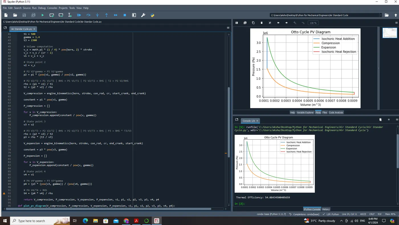
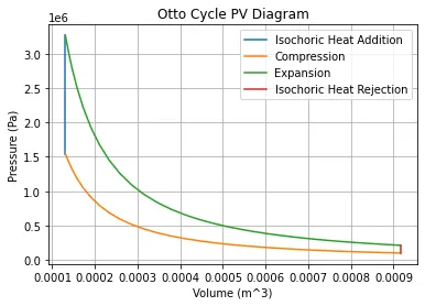 Thermal Efficiency: 54.08434500405659
Conclusion:
The PV diagram obtained visually illustrates the thermodynamic sequences inherent in the air-standard Otto cycle. This graph offers insights into alterations in pressure and volume across the cycle's four stages: compression, constant volume heat addition, expansion, and constant volume heat rejection. The computed thermal efficiency (approximately 55%) reflects the engine's efficiency in converting heat energy into useful work during the cycle. This efficiency is quantified as the ratio between the area enclosed by the expansion and compression curves and the area beneath the constant volume heat addition and rejection lines. The PV diagram vividly depicts the cyclic progression of the Otto cycle, elucidating the sequence of thermodynamic phases experienced by the engine. The enclosed region within the curve encapsulates the overall work output generated by the engine in a single cycle.