Week 2 Air standard Cycle

Aim: To write a program in python to generate a theoretical and an actul P-V diagram of an Otto cycle and also find the thermal efficiency of the engine.

Theory: Otto cycle is basically a thermodynamic cycle which is used in the analysis petrol engines. Four types of processes take place when we're considering a 4-stroke IC engine and they're: Intake or suction stroke,compression stroke,expansion stroke and exhaust stroke. It is an air standard cycle because the working fluid which is involved is specifically air. He're while writing the code of the following otto cycle, we're basically considering only the compression and expansion process, and how the volume variation is taking place iniside the engine cylinder, and it's corresponding effect on the pressure.

The assumptions of the air standard cycle are :
(1)The gas in the engine cylinder is assumed to be perfect.

(2)Compression and expansion processes that take place inside the engine cylinder are assumed to be reversible and adiabatic.

(3)The cycle is considered to be taking place in a closed system with no air leaving or entering into the system.

The compression and expansion that we're considering here involves 4 state points.

1-2: Reversible adiabatic compression
2-3: Constant volume heat addition
3-4: Reversible adiabatic expansion
4-1: Constant volume heat rejection

The major thermodynamic equations involved are :

pv^γ=C and pv/T=C

where p-pressure,v-volume ,T-temperature, C-constant and gamma is the adiabatic index. These equations helps us to calculate p,v and T at all four state points.

Also, the piston kinematics equation drives the volume variation during compression and expansion strokes and is given by:

V=Vc*[(1+0.5(cr-1)*[R+1-cos(theta)-(R^2-sin^2(theta))^0.5]]

where V-stroke volume,cr-compression ratio,R-ratio of connecting rod length to crank pin radius,theta-crank angle and Vc-clearance volume. As theta chnages, V changes. All other factors are constant in the equation.

Procedure:

1)We firstly assign the pressure and temperature at state point 1 as p1=101325 atm and t1= 500 K respectively. From coding point of view, we don't provide the units.

2)The temperature at the end of combustion which is the maximum temperature achieved inside cylinder is assigned t3=2300K.

3)The volume inside a cylinder doesn't vary linearly. Rather, it depends on the engine geometric parameters and is driven by the piston kinematics equation. Engine geometric parameters include bore diameter,stroke length,connecting rod length and compression ratio. The values are assigned as : bore_dia=0.1,stroke=0.1,con_rod=0.15 and cr=12.

4)Then, we define the formulae used to calculate swept volume and clearance volume. Swept volume is the volume covered by piston movement from TDC to BDC and is given by vs=(M.pi/4)*(bore_dia*bore_dia)*stroke. Clearance volume is the volume above TDC beyond which piston can't move and is given by vc=vs/(cr-1).

5)Now , the volume v1=(vs+vc) which is nothing but the total volume. v2=vc since the value of clearance volume is assigned to v2. Since we know the p1,v1 and t1 values at state point 1, we then go on to find the p2 and T2 values, at state point 2. We write : p2=p1*pow(cr,gamma) which is through using the equation pv^gamma=C and calculate p2. Then, we find out t2=(p2*v2*t1)/(p1*v1) by using PV/T = C equation.

6)Similarly, we go on to find p3,v3and t3 for the expansion process and state point 3 and also the v4,p4and t4 for state point 4. Note that, since process 2-3 is constant volume heat addition , hence v3=v2. Also, since process 4-1 is constant volume heat rejection, hence v4=v1.

7)Now that we have calculated p,v,t at all the state points,we then create a user-defined function using the following syntax: def eng_kinematics(bore_dia,stroke,con_rod,cr,start_crank,end_crank): where def-keyword is used to create a user defined function,eng_kinematics is the function name and all factors inside the bracket are the input arguments. This function is defined so that we can calculate the volume variation which is basically a function of crank angle.

8)Inside the function , we calculate a=stroke/2,R=con_rod/a,vs and vc as well. The start_crank and end_crank values are stored in sc and ec in radians. That is why, we write : sc=M.radians(start_crank) and ec=M.radians(end_crank). We then define the crank angle using variable theta = np.linspace(sc,ec,50) and create an array of 50 different crank angle values in radians. We then create an empty array of v using the command v=[] where we would be storing the multiple values of volume corresponding to 50 different theta values.

9)We then finally create a for loop so that we can access each crank angle value and hence we write : Theta= theta[i] and calculate the stroke volume continuously for 50 times for 50 different crank angle values using the piston kinematics equation which has been mentioned already in the theory part. And finally we're using the append command to add all the values of v(stroke volume) calculated into the empty array v. Since, we're looking for the output of the function to be v, that is why we write : return v. This is the entire function definition portion which is defined in points 7,8,9.

10)Then, we move to function calling part. We do it using the command V_comp=eng_kinematics(bore_dia,stroke,con_rod,cr,180,0) where engine geometric parameters are constant .Only start_crank and end_crank values are mentioned as 180,0 as we're calculating the volume values during compression process for different crank angle values and those volume values are stored in V_comp. We then run a for loop to store each V_comp value in j so that for each V_comp value, we can find out corresponding P_comp values. For that, we use an empty P_comp array using P_comp=[] and append function to finally store all values. Also, value of constant C is calculated before calculating P_comp values for corresponding V_comp. We follow a similar approach for doing the same with the expansion process. Just that during expansion process, start_crank and end_crank values will be 0 ,180 respectively as opposed to 180,0 during compression.

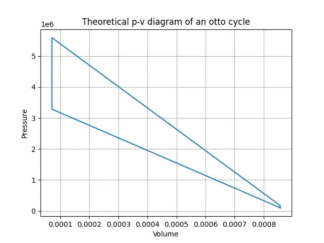
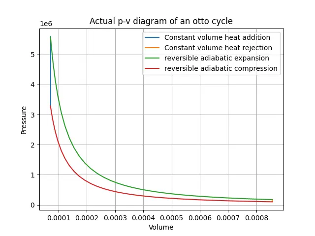
11) Finally, we plot two types of p-v diagram of otto cycle. One is the theoretical p-v diagram and other is the actual p-v diagram using plot command like plt.plot(x,y). We provide xlabel,ylabel and title using the plt.xlabel,plt.ylabel and plt.title commands respectively. We create 2 separate figures using the plt.figure() command. In the theoretical p-v diagram, the volume variation is linear as we're simply joining all the four state points but not considering the piston kinematics equation. In actual p-v diagram, the volume variation is non-linear and is driven by piston kinematics equation for which we have actually written the user-defined function.

12)The thermal efficiency of the engine has also been calculated using the formula:1-[(t4-t1)/(t3-t2)]. From coding point of view, we have used a variable Th_eff=1-(t4-t1)/(t3-t2) to calculate the thermal efficiency.

The scripting of the code is pasted below:

import math as M
import numpy as np
import matplotlib.pyplot as plt

#User-defined function to calculate the volume variation during compression and expansion process using piston kinematics equation
def eng_kinematics(bore_dia,stroke,con_rod,cr,start_crank,end_crank):
    a=stroke/2
    R=con_rod/a
    vs=M.pi*(1/4) *pow(bore_dia,2)*stroke
    vc=vs/(cr-1)

    sc=M.radians(start_crank)
    ec=M.radians(end_crank)

    theta=np.linspace(sc,ec,50)
    
    v=[]
    
    for i in range(0,50):
        Theta=theta[i]
        term1=0.5*(cr-1)
        term2=R+1-M.cos(Theta)
        term3=pow(R,2)-pow(M.sin(Theta),2)
        term3=pow(term3,0.5)
        v.append((1+term1*(term2-term3))*vc)
    return v

#Engine geometric parameters
bore_dia=0.1
stroke=0.1
con_rod=0.15
cr=12
gamma=1.4

#Pressure and temperature values
p1=101325
t1=500
t3=2300

#Calculation of swept volume and clearance volume
vs=(M.pi/4)*(bore_dia*bore_dia)*stroke
vc=vs/(cr-1)
v1=vs+vc
v2=vc

p2=p1*pow(cr,gamma)
t2=(p2*v2*t1)/(p1*v1)

#Calling the function for compression process
V_comp=eng_kinematics(bore_dia,stroke,con_rod,cr,180,0)
C=p1*pow(v1,gamma)
P_comp=[]

for j in V_comp:
    P_comp.append(C/pow(j,gamma))
    

v3=v2
p3=(p2*t3)/t2


#Calculation of p4,v4,t4
v4=v1
p4=p3*pow((v3/v1),gamma)
t4=(p4*v4*t3)/(p3*v3)

Th_eff=1-(t4-t1)/(t3-t2)
print(Th_eff)
#Calling the function for expansion process
V_power=eng_kinematics(bore_dia,stroke,con_rod,cr,0,180)
C=p3*pow(v3,gamma)
P_power=[]

for k in V_power:
    P_power.append(C/pow(k,gamma))
    

#Plotting the theoretical pv- diagram
plt.figure()
plt.plot([v1,v2,v3,v4,v1],[p1,p2,p3,p4,p1])
plt.xlabel('Volume')
plt.ylabel('Pressure')
plt.title('Theoretical p-v diagram of an otto cycle')
plt.grid()
plt.show()

#Plotting the Actual pv-diagram 
plt.figure()
plt.plot([v2, v3],[p2, p3])
plt.plot([v4, v1],[p4, p1])
plt.plot(V_power, P_power)
plt.plot(V_comp, P_comp)
plt.xlabel('Volume')
plt.ylabel('Pressure')
plt.title('Actual p-v diagram of an otto cycle')
plt.legend(['Constant volume heat addition','Constant volume heat rejection','reversible adiabatic expansion','reversible adiabatic compression'])
plt.grid()
plt.show()

The output graphs are pasted below:

Conclusion:

The plot 1 shows a theoretical p-v diagram of the otto cycle as we can clearly see that volume is varying linearly during compression and expansion process.

The plot 2 represents the actual p-v diagram of an otto cycle as we can see that the volume variation during compression and expansion process is non-linear and curved and driven by piston kinematics equation. However, the constant volume heat addition and rejection processes remains constant in both the plots.