Week 3 - Solving second order ODEs

Aim: To write a program in Python that simulates the motion of a simple pendulum with damping and is basically governed by a second order ODE given by :

(d^2 )θ/(dt^2 )+(b/m)dθ/dt+(g/L)sinθ=0

where g-acceleration due to gravity in m/s^2,L-length of the pendulum in m,m-mass of the ball in kg and b-damping coefficient.

Theory: A simple pendulum basically consists of a mass m which in this case is the ball of 1kg,hanging from a string of length l which is 1 m and fixed at a pivot point on the other side. The way the pendulum moves depends on Newtons second law. When this law is written down,we get a second order ODE that describes the position of ball w.r.t time. In the code, we have broken down the second order ODE into two first order ODE's and then proceeded,as the solver odeint can solve first order ODE's only. ODE's are used to describe the transient behaviour of a system which in this case is a simple pendulum system.

Procedure:

1) Firstly, we import all necessary modules. numpy module is imported as we're creating an array of time using linspace command. scipy library is imported as it contains odeint which is used to solve ODEs in python. math module is imported as we have calculated certain parameters like x1,y1 and dtheta_2dt which involves use of sine and cosine. Lastly,matplotlib is imported as we have used the multiple plot commands.

2) Then we initialise the variables b,g,l and m as 0.05,9.81,1 and 1 respectively. These are constants in the program.

3) We then provide initial conditions through the variable theta_0. We have written theta_0=[0,3] to provide the initial conditions as initial angular displacement=0 and initial angular velocity =3. Also, we have defined the time array using linspace command for 0-20s as that is the time we're supposed to simulate the simple pendulum system for.

4) We have then written the most important part i.e. scripting the user-defined function. The user defined function is created using def keyword and the name of the function is simple_pendulum. The input arguments are solution variable theta,time-t,b,g,l,m. The solution variable theta outputs two columns, first is the angular displacement values for 80 different values of time and second column is the angular velocity values for 80 different values of time. It is simulated for 20s. theta1 contains first column of solution variable theta, and theta2 contains second column. That is defined when we have written: theta1=theta[0] and theta2=theta[1].

We have then written down the two linear algebraic forms of the ODE which we have converted. This is called discretization. dtheta1_dt=theta2 and dtheta2_dt=-9b/m)*theta2-(g/l)*M.sin(theta1) are the two algebraic equations which we have used. dtheta_dt is the output of the function which we want and hence we're writing return dtheta_dt.

5) We then go on to calculate the solution of the equations using odeint solver which is used to solve ODEs in python. The solution is stored in variable theta and function name,theta_0,t,args=b,g,l,m are the inputs provided to the solver and is a part of syntax of odeint.

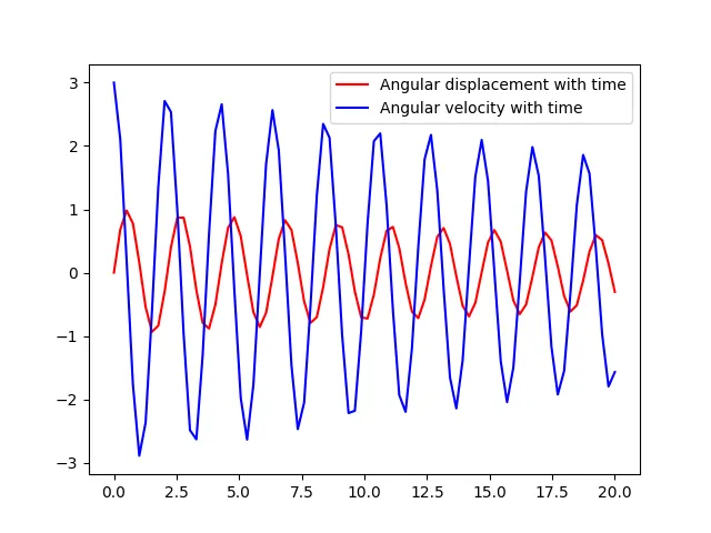
6) Finally, we go on to plot the angular displacement w.r.t time curve and angular velocity w.r.t time curve. We're doing this by writing plt.plot(t,theta[:,0]) for displacement-time curve and plt.plot(t,theta[:,1]) for velocity-time curve. Also, we have provided the red color and blue color respectively for the plots. The legends are also provided to differentiate the curves.

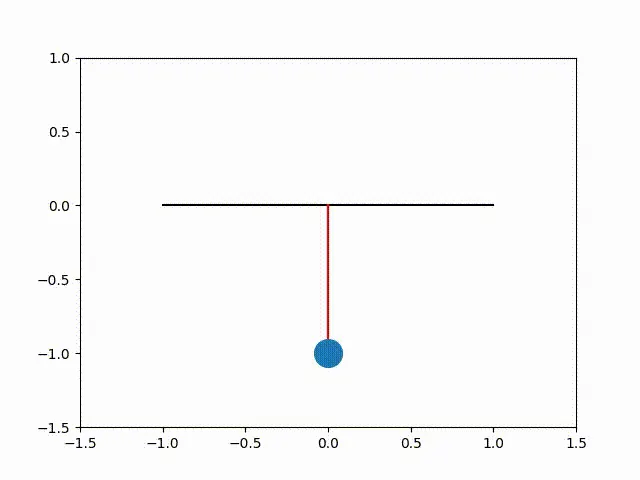
7) We then run a for loop where we calculate the x1,y1 coordinates by writing x1=l*M.sin(i) and y1=-l*M.cos(i). The negative sign in y1 is provided as we want the ball to be swinging in the 3rd and 4th quadrant and in negative y-axis. We're doing this so that for every value of angular displacement, we can plot the respective positions of the ball as a function of time. plt.plot([x0,x1],[y0,y1]) is used to create the part which is length of the string and plt.plot(x1,y1,'o',markersize=20) creates the centre of the ball with a certain diameter which we have done using markersize command. Also, xlimit and ylimit are also provided.

8) The images which we have created have been saved in the variable filename and ct is the counter variable we have used to save images with the right name. plt.savefig(filename) saves all the images with the correct name in order. After getting all images, we just stiched all images and converted into a gif/video file.

Errors:

1. If we don't provide the x-limit and y-limit, certain positions go out of frame and can't be seen.

2. When we have considered time array from 0-20s and taken 20 points, the images are not that coherent and smoothness of the animation is not maintained in that case and even the ball swings in 1st quadrant as well which goes above the x-axis. This is rectified when we have considered 100 points in time array and in turn the animation is also much more fluid.

import numpy as np
from scipy.integrate import odeint
import math as M
import matplotlib.pyplot as plt

#Initialising the variables
b=0.05
g=9.81
l=1
m=1

#Providing initial conditions
theta_0=[0,3]
t=np.linspace(0,20,80)

# Scripting user defined function
def simple_pendulum(theta,t,b,g,l,m):
    theta1=theta[0]
    theta2=theta[1]
    dtheta1_dt=theta2
    dtheta2_dt=-(b/m)*theta2-(g/l)*M.sin(theta1)
    dtheta_dt=[dtheta1_dt,dtheta2_dt]
    return dtheta_dt

theta=odeint(simple_pendulum,theta_0,t,args=(b,g,l,m))
print(theta)


plt.plot(t,theta[:,0],color='r',label='Angular displacement with time')
plt.plot(t,theta[:,1],color='b',label='Angular velocity with time')
plt.legend()

ct= 101
x0=0
y0=0
for i in theta[:,0]:
    x1=l*M.sin(i)
    y1=-l*M.cos(i)
    filename=str(ct)+'.png'
    ct=ct+1

    plt.figure()
    plt.plot([-1,1],[0,0],'black')
    plt.plot([x0,x1],[y0,y1],'red')
    plt.plot(x1,y1,'o',markersize='20')
    plt.xlim([-1.5,1.5])
    plt.ylim([-1.5,1])
    plt.savefig(filename)
    plt.show()

The animation file is pasted below:

The displacement time curve and velocity time curve are in the same figure provided with legends. The angular velocity varies more as a function of time compared to angular displacement. By this it means, the peak positive and negative values are much greater for angular velocity compared to angular displacement.