Week 5 - Curve fitting

Ans 1. popt is basically an array that stores the value of coefficients a and b in case of a linear polynomial equation or it stores the value of coefficients a,b,c,d in case of a cubical polynomial equation.
pcov is a covariant matrix where if the degree of polynomial (n) is 1 in case of linear polynomial equation, the matrix will be a 2-by-2 or of the type (n+1)-by-(n+1). Similarly, if we're assuming a cubical polynomial equation where degree (n) is 3, then the covariant marix pcov will be of the type 4-by-4.

Ans 2. np.array(temperature) considers all the values of temperature array provided in the data file, and not a single value of temperature array.

Ans 3. The * in *popt indicates that all the values of coefficients are being considered which are calculated , and not any specific coefficient value.

Ans 4.

AIM: To write a code in python to fit a linear and cubic polynomial for the Cp data provided.

THEORY: Curve-fitting is a technique used in data analysis to establish a mathematical relationship between x and y data. In this case, x-temperature and y-specific heat. x-independent variable,y-dependent variable.

4.1 PROCEDURE for code 1(Linear curve fit):

1. Firstly, we're importing the modules like math,numpy,matplotlib and curve_fit module from scipy library.

2. Then,we go on to load the data from the data file provided by writing a user-defined function by the name read_file(). We consider an empty array of temperature and cp. After that, a for loop is run to extract line-by-line data from the data file. We're then using split command to separate the temperature and cp data which are separated by comma(,). Finally, we're using append command to add all the temperature and cp data into their respective empty arrays. Then, we're writing return[tempearature,cp] as output of the function read_file(). Now, we're calling the function read_file and finally all the data from data file is stored and extracted into the temperature and cp arrays.

3. We assume the linear polynomial equation after that using a user-defined function by the name linear and written as def linear(T,a,b): and return the output of the function as a*T+b which is the linear equation.

4. Then, we go on to calculate the coefficients of the linear equation by using curve_fit command when we're writing: popt,pcov=curve_fit(linear,temperature,cp) where linear is the function name,temperature is the x-data and cp is the y-data and popt,pcov are already described above what they mean.

5. Then, the predicted cp values are calculated in the variable predicted_cp. We're then calling the user-defined function we've written for assuming the linear polynomial equation. Here, predicted_cp=linear(np.array(temperature),*popt) where linear is the function name,np.array(temperature) are all the temperature values passed in input arguments for calculating 3200 predicted_cp values and *popt is the values of all coefficients which we have already calculated.

6. The goodness of the fit is then calculated and found out to be : 0.9248776260524184 which is the R-square parameter calculation. The fitness of the curve is not good as, if we're considering cubic polynomial equation as in next case, the R-square parameter=0.9967259467146888 which is much greater as compared to the linear-fit R-square parameter. So, in the contrary this fit can be considered to be bad.

7. Finally ,we 're just plotting the original data which is temperature vs Cp data , and the curve-fit data which is temperature vs predicted_cp data using plot commands, and giving it a color,linewidth and appropriate legends.

The code 1 pasted below:

import math as M
import numpy as np
import matplotlib.pyplot as plt
from scipy.optimize import curve_fit

# Writing a function for loading the data file into python
def read_file():
    temperature=[]
    cp=[]
    for line in open('data','r'):
        values=line.split(',')
        temperature.append(float(values[0]))
        cp.append(float(values[1]))
    return [temperature,cp]

def linear(T,a,b):
    return a*T+b

[temperature,cp]=read_file()
#print(cp)

#Calculating coefficients a and b
popt, pcov = curve_fit(linear,temperature,cp)

#Calculating predicted_cp
predicted_cp=linear(np.array(temperature), *popt)

#R^2 parameter/goodness of fit calculation
A=pow((np.array(np.array(cp)-np.array(predicted_cp))),2)
SSE=np.sum(A)
B=np.mean(cp)
C=pow((np.array(np.array(predicted_cp)-B)),2)
SSR=np.sum(C)
SST=SSE+SSR
R_square= SSR/SST
print(R_square)

#Plotting
plt.figure()
plt.plot(temperature,cp,color='b',linewidth=3)
plt.plot(temperature,predicted_cp,color='r',linewidth=3)
plt.xlabel('Temperature[T]')
plt.ylabel('Specific heat[Cp]')
plt.legend(['Original data','curve-fitted data'])
plt.show()

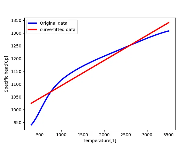
Plot 1: This plot above shows the curve fit data when we're considering a linear polynomial equation. And, as per the R-square value which is found out to be 0.9248776260524184, we can definitely say the fitness of the curve is not good or bad. Also, by visual observation we can say that the curve fit data when assuming a linear polymial equation is not a good fit in this case.

4.2 PROCEDURE for code 2(Cubical curve fit):

1. Firstly, we're importing the modules like math,numpy,matplotlib and curve_fit module from scipy library.

2. Then,we go on to load the data from the data file provided by writing a user-defined function by the name read_file(). We consider an empty array of temperature T and cp. After that, a for loop is run to extract line-by-line data from the data file. We're then using split command to separate the temperature and cp data which are separated by comma(,). Finally, we're using append command to add all the temperature and cp data into their respective empty arrays. Then, we're writing return[T,cp] as output of the function read_file(). Now, we're calling the function read_file and finally all the data from data file is stored and extracted into the T and cp arrays.

3. We assume the cubical polynomial equation after that using a user-defined function by the name cubic_eqn and written as def cubic_eqn(t,a,b): and return the output of the function as a*pow(t,3)+b*pow(t,2)+c*t+d which is the cubical polynomial equations. t,a,b are inputs for the function.

4. Then, we go on to calculate the coefficients of the cubical equation by using curve_fit command when we're writing: popt,pcov=curve_fit(cubic_eqn,T,cp) where cubic_eqn is the function name,T is the x-data and cp is the y-data and popt,pcov are already described above what they mean.

5. Then, the predicted cp values are calculated in the variable pr_cp. We're then calling the user-defined function we've written for assuming the cubic polynomial equation. Here,pr_cp=cubic_eqn(np.array(T),*popt) where cubic_eqn is the function name,np.array(T) are all the temperature values passed in input arguments for calculating 3200 pr_cp values and *popt is the values of all coefficients which we have already calculated.

6. The goodness of the fit is then calculated and found out to be : 0.9967259467146888 which is the R-square parameter calculation. The fitness of the curve is good as, if we're considering linear polynomial equation as in previous case, the R-square parameter=0.9248776260524184 which is much lower as compared to the cubical-fit R-square parameter. So, in the contrary this fit can be considered to be good.

7. Finally ,we 're just plotting the original data which is T vs Cp data , and the curve-fit data which is T vs pr_cp data.

The code 2 pasted below:

import numpy as np
import math as M
import matplotlib.pyplot as plt
from scipy.optimize import curve_fit

# user-defined function to load the data from data file

def read_file():
    T=[]
    cp=[]
    for line in open('data','r'):
        values=line.split(',')
        T.append(float(values[0]))
        cp.append(float(values[1]))
    return [T,cp]

def cubic_eqn(t,a,b,c,d):
    return a*pow(t,3)+b*pow(t,2)+c*t+d

T,cp=read_file()

#Calculating coefficients a,b,c and d
popt,pcov=curve_fit(cubic_eqn,T,cp)

#Calculating predicted_cp
pr_cp=cubic_eqn(np.array(T),*popt)

#Calculation of R^2 parameter/goodness of fit
A=pow((np.array(np.array(cp)-np.array(pr_cp))),2)
SSE=np.sum(A)
B=np.mean(cp)
C=pow((np.array(np.array(pr_cp)-B)),2)
SSR=np.sum(C)
SST=SSE+SSR
R_square=SSR/SST
print(R_square)

#Plotting
plt.figure()
plt.plot(T,cp,color='b',linewidth=3)
plt.plot(T,pr_cp,color='r',linewidth=3)
plt.xlabel('Temperature[T]')
plt.ylabel('Specific heat[Cp]')
plt.legend(['Original data','curve-fitted data'])
plt.show()

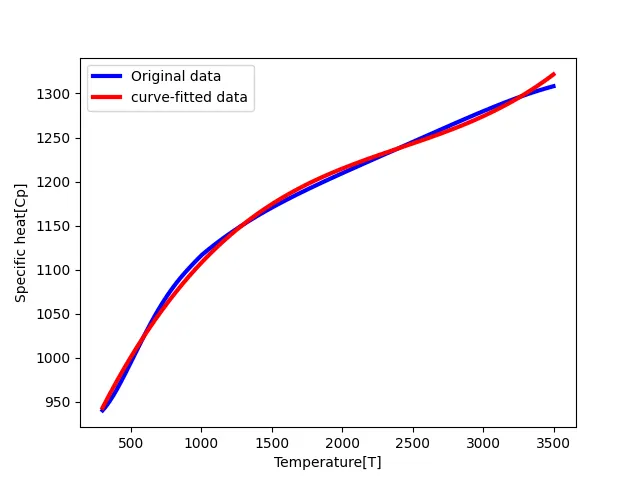
Plot 2: This plot above shows the curve fit data when we're considering a cubical polynomial equation. And, as per the R-square value which is found out to be 0.9967259467146888 , we can definitely say the fitness of the curve is good as compared to previous case. Also, by visual observation we can say that the curve fit data when assuming a cubical polymial equation is a good fit in this case.

4.3 PROCEDURE for code3(Splitwise-polynomial curve fit):

1. Firstly, we're importing the modules like math,numpy,matplotlib and curve_fit module from scipy library.

2. Then,we go on to load the data from the data file provided by writing a user-defined function by the name read_file(). We consider an empty array of temperature T and cp. After that, a for loop is run to extract line-by-line data from the data file. We're then using split command to separate the temperature and cp data which are separated by comma(,). Finally, we're using append command to add all the temperature and cp data into their respective empty arrays. Then, we're writing return[T,cp] as output of the function read_file(). Now, we're calling the function read_file and finally all the data from data file is stored and extracted into the T and cp arrays.

3. We create 4 different functions for all the 4 different ranges which we have converted temperature and cp data into. The first function is func for range 1 and assumed a linear polynomial, second function is func1 for range 2 and assumed a cubic polynomial, third function is func2 for range 3 and assumed a cubic polynomial again and the last function is func3 for range 4 and again assumed a linear polynomial. And, obviously linear equations are given by a*t+b where a and b are coefficients,t is the x-data which is temperature and cubical equations given by a*pow(t,3)+b*pow(t,2)+c*t+d where there are 4 coefficients a,b,c and d, and t-is the x-data which is temperature.

4. We're now dividing the entire temperature T and specific heat cp data into 4 different ranges. For range 1, temp1=np.array(T[0:800]) means we're considering the first 800 rows of the temperature or T data. Similarly, cp1=np.array(cp[0:800]) means we're considering the first 800 values of cp data. For range 2, temp2=np.array(T[800:1600]) means we're considering the values from 800-1600 rows of the temperature or T data. Similarly, cp2=np.array(cp[800:1600]) means we're considering the values from 800-1600 rows of cp data. For range 3, temp3=np.array(T[1600:2400]) means we're considering the values from 1600-2400 rows of the temperature or T data. Similarly, cp3=np.array(cp[1600:2400]) means we're considering the values from 1600-2400 rows of cp data. For range 4, temp4=np.array(T[2400:3200]) means we're considering the values from 2400-3200 rows of the temperature or T data. Similarly, cp4=np.array(cp[2400:3200]) means we're considering the values from 2400-3200 rows of cp data. This is what we're doing differently in splitwise polynomial.

5. For all the different ranges from 1-4, popt and pcov are calculated separately. popt,pcov used to calculate coefficients for range 1 linear polynomial,popt1,pcov1 used to calculate coefficients for range 2 cubic polynomial, popt2,pcov2 used to calculate coefficients for range 3 cubic polynomial and popt3,pcov3 used to calculate coefficients for range 4 which is linear polynomial. All the coefficient calculations are done using curve_fit command and then passing the function name, and respective temperature and cp data ranges.

6. pr_cp1,pr_cp2,pr_cp3 and pr_cp4 are the four different predicted cp values for range 1,range 2,range 3 and range 4 respectively. For predicted cp calculation, we're just calling the function name and passing the corresponding range of temperature data like np.array(temp1) for range 1,np.array(temp2) for range 2,np.array(temp3) for range 3 and np.array(temp4) for range 4 along with all the coefficients using *popt,*popt1,*popt2,*popt3 for the respective ranges.

7. We then go on to plot the original data first which is done using plt.plot(T,cp). Then, we go on to plot the temp1 vs pr_cp1 data for range 1 using plt.plot(temp1,pr_cp1) and giving it a blue color. We do the same for other 3 ranges as well in order and giving it the green,black and violet colors respectively. The keyword label is used to provide the legend names and then finally calling it like this where we write plt.legend(). We also provide the x-label and y-label to make the graph look authentic and practical.

8. Finally, we do the R-square parameter calculation for different ranges and is done in the same manner as we have done in code 1 and code 2. Just that, out here we have considered 4 different equations for 4 different ranges and hence, 4 separate R-square values are found out separately for the respective ranges.

The code 3 is pasted below:

import math as M
import numpy as np
import matplotlib.pyplot as plt
from scipy.optimize import curve_fit

# Writing user-defined function to load the data
def read_file():
    T=[]
    cp=[]
    for line in open('data','r'):
        values=line.split(',')
        T.append(float(values[0]))
        cp.append(float(values[1]))
    return [T,cp]

T,cp = read_file()

#Assuming polynomial equation for range 1
def func(t,a,b):  #Function for range 1
    return a*t+b

def func1(t,a,b,c,d): #Function for range 2
    return a*pow(t,3)+b*pow(t,2)+c*t+d

def func2(t,a,b,c,d):  #function for range 3
    return a*pow(t,3)+b*pow(t,2)+c*t+d

def func3(t,a,b):   #function for range 4
    return a*t+b

#range 1
temp1=np.array(T[0:800])
cp1=np.array(cp[0:800])
#Calculation of coefficients for range 1
popt, pcov=curve_fit(func,temp1,cp1)
#Calculation of predicted_cp for range 1
pr_cp1=func(np.array(temp1),*popt)


#range 2
temp2=np.array(T[800:1600])
cp2=np.array(cp[800:1600])
#calculation of coefficients for range 2
popt1,pcov1 = curve_fit(func1,temp2,cp2)
#calculation of predicted_cp for range 2
pr_cp2=func1(np.array(temp2),*popt1)


#range 3
temp3=np.array(T[1600:2400])
cp3=np.array(cp[1600:2400])
#range 3 coefficients calculation
popt2,pcov2=curve_fit(func2,temp3,cp3)
# Calculation of predicted cp for range 3
pr_cp3=func2(np.array(temp3),*popt2)


#Range 4
temp4=np.array(T[2400:3200])
cp4=np.array(cp[2400:3200])
#range 3 coefficients calculation
popt3,pcov3=curve_fit(func3,temp4,cp4)
# Calculation of predicted cp for range 3
pr_cp4=func3(np.array(temp4),*popt3)


plt.figure()
#Plotting for range 1
plt.plot(T,cp,color='r',linewidth=3,label='original data')

plt.plot(temp1,pr_cp1,color='b',linewidth=3,label='curve-fit data-range 1')
#Plotting for range 2
plt.plot(temp2,pr_cp2,color='g',linewidth=3,label='curve-fit data-range 2')

#Plotting for range 3
plt.plot(temp3,pr_cp3,'black',linewidth=3,label='curve-fit data-range 3')

#Plotting for range 4
plt.plot(temp4,pr_cp4,'violet',linewidth=3,label='curve-fit data-range 4')

plt.xlabel('Temperature[T]')
plt.ylabel('Specific heat[cp]')

plt.legend()
plt.show()

#R-square calculation for range 1
A1=pow((np.array(np.array(cp1)-np.array(pr_cp1))),2)
SSE1=np.sum(A1)
B1=np.mean(cp1)
C1=pow((np.array(np.array(pr_cp1)-B1)),2)
SSR1=np.sum(C1)
SST1=SSE1+SSR1
R_square1=SSR1/SST1
print("R-square 1=",R_square1)

#R-square calculation for range 2
A2=pow((np.array(np.array(cp2)-np.array(pr_cp2))),2)
SSE2=np.sum(A2)
B2=np.mean(cp2)
C2=pow((np.array(np.array(pr_cp2)-B2)),2)
SSR2=np.sum(C2)
SST2=SSE2+SSR2
R_square2=SSR2/SST2
print("R-square 2=",R_square2)

#R-square calculation for range 3
A3=pow((np.array(np.array(cp3)-np.array(pr_cp3))),2)
SSE3=np.sum(A3)
B3=np.mean(cp3)
C3=pow((np.array(np.array(pr_cp3)-B3)),2)
SSR3=np.sum(C3)
SST3=SSE3+SSR3
R_square3=SSR3/SST3
print("R-square 3=",R_square3)

#R-square calculation for range 4
A4=pow((np.array(np.array(cp4)-np.array(pr_cp4))),2)
SSE4=np.sum(A4)
B4=np.mean(cp4)
C4=pow((np.array(np.array(pr_cp4)-B4)),2)
SSR4=np.sum(C4)
SST4=SSE4+SSR4
R_square4=SSR4/SST4
print("R-square 4=",R_square4)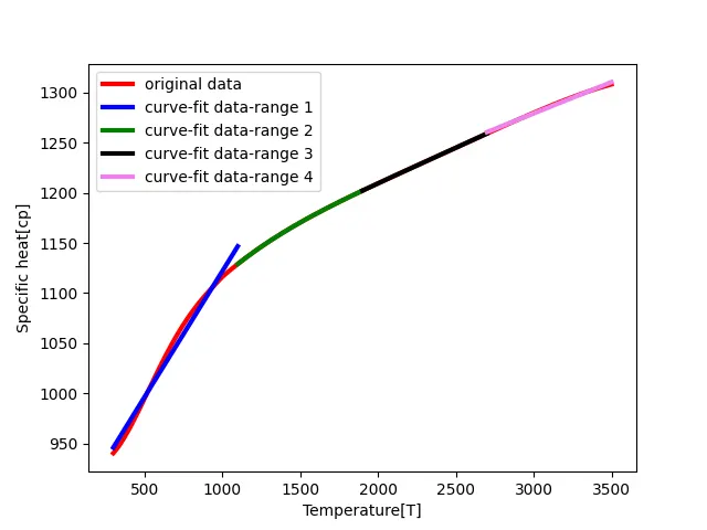

Plot 3: This plot above shows the curve fit data when we're considering a linear polynomial equation for range 1, cubic polynomial equation for range 2, cubic polynomial equation for range 3, and a linear polynomial equation again for range 4. For range 1, R-square value = 0.9845086679691486, for range 2,R-square=0.9999997086207656, for range 3,R-square=0.9999995300425422 and for range 4,R-square=0.996882030634896. We can say that the goodness of fit is really good for range 2 and 3 considering cubic polynomial equation. For range 4, it is fairly good considering the linear polynomial,we can say. For range 1, it is bad and linear polynomial is not a good fit.

ANS 5: In order for the curve to fit perfect, we can:

(i) Either increase the degree of polynomial that also further increases the complexity of calculation. Moreover, due to that we have seen that a cubic polynomial gives a better curve fit than linear one.

(ii)Splitwise polynomial gives best curve fit in contrary to single type be it linear or cubic polynomial.

ANS 6: It has already been explained through respective R-square parameter calculation separately in plot section of all three codes.