Week 2 Air standard Cycle

AIM :

write code that can solve an otto cycle and make plots for it.

Here are the requirements

1. Your code should create a PV diagram

2. You should output the thermal efficiency of the engine.

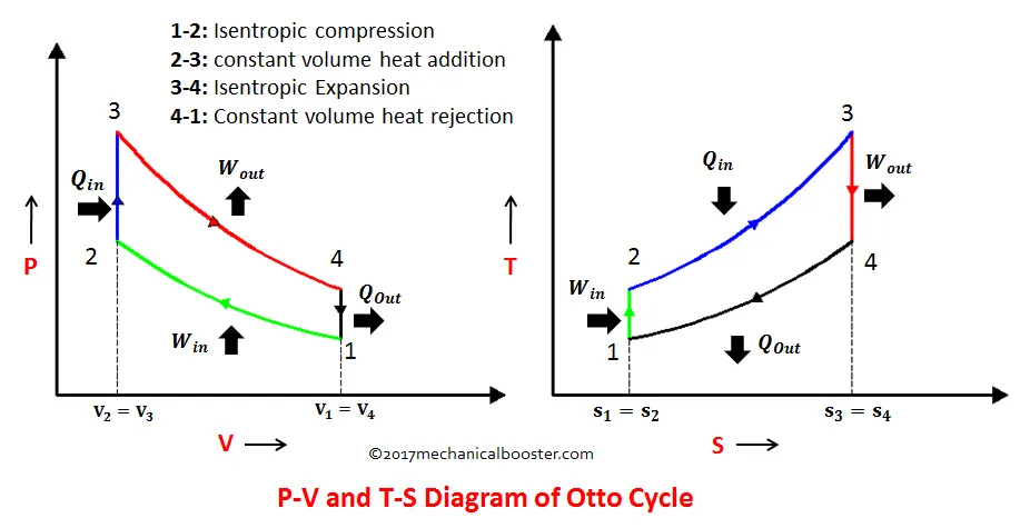
Otto cycle is also termed as a constant volume power cycle. It contains a pair of isentropic processes and a pair of isochoric processes. This cycle basically used for spark ignition engines.

s shown in figure red and green lines indicate the isentropic compression and expansion respectively and blue and black lines indicate the constant volume heat addition.

The Otto cycle contains 4 state processes:-

• Process 1-2 Isentropic compression
• Process 2-3 constant volume heat addition
• Process 3-4 isentropic expansion
• Process 4-1 constant volume heat rejection

The processes are described by

• Process 0–1 a mass of air is drawn into piston/cylinder arrangement at constant pressure.
• Process 1–2 is an adiabatic (isentropic) compression of the charge as the piston moves from bottom dead center (BDC) to top dead center (TDC).
• Process 2–3 is a constant-volume heat transfer to the working gas from an external source while the piston is at top dead center. This process is intended to represent the ignition of the fuel-air mixture and the subsequent rapid burning.
• Process 3–4 is an adiabatic (isentropic) expansion (power stroke).
• Process 4–1 completes the cycle by a constant-volume process in which heat is rejected from the air while the piston is at bottom dead center.
• Process 1–0 the mass of air is released to the atmosphere in a constant pressure process.

The Otto cycle consists of isentropic compression, heat addition at constant volume, isentropic expansion, and rejection of heat at constant volume. In the case of a four-stroke Otto cycle, technically there are two additional processes: one for the exhaust of waste heat and combustion products at constant pressure (isobaric), and one for the intake of cool oxygen-rich air also at constant pressure; however, these are often omitted in a simplified analysis. Even though those two processes are critical to the functioning of a real engine, wherein the details of heat transfer and combustion chemistry are relevant, for the simplified analysis of the thermodynamic cycle, it is more convenient to assume that all of the waste-heat is removed during a single volume change.

INPUTS:

• gamma = adiabatic index
• stoke = stroke length of the connecting rod
• bore = bore diameter of the cylinder
• con_rod = length of the connecting rod
• cr = compression ratio
• v_swept = swept volume of the cylinder
• v_clearance = clearance volume of the cylinder
• theta = crank angle
• v = volume of the cylinder
• e = thermal efficiency of the engine
• p1,v1,t1 = corresponding pressure,volume and temperature at point 1
• p2,v2,t2 = corresponding pressure,volume and temperature at point 2
• p3,v3,t3 = corresponding pressure,volume and temperature at point 3
• p4,v4,t4 = corresponding pressure,volume and temperature at point 4

EQUATIONS USED IN THE PPROGRAM :

1. v_swept = (pi/4)*bore^2*stroke
2. v_clearance = v_swept/(cr-1)
3. constant = p*v^gamma
4. p*v = constant_c*t
5. a = stroke/2
6. R = con_rod/a
7. v/v_c = (1 + 0.5*(cr-1)*(R + 1 - cos(theta) -( R^2 -sin(theta))^0.5))
8. e = 1- 1/[cr^(gamma-1)]

GENERATE PROGRAM DESCRIBES OTTO CYCLE :

# cyclone simulattor

import  math
import matplotlib.pyplot as plt 


def engine_kinematics(bore,stroke,con_rod,cr,start_crank,end_crank):

	# geometric parameters
	
	a = stroke/2
	R = con_rod/a

	v_s = math.pi*(1/4)*pow(bore,2)*stroke
	v_c = v_s/(cr-1)

	sc = math.radians(start_crank)
	ec = math.radians(end_crank)

	num_values = 50

	dtheta = (ec-sc)/(num_values-1)

	V = []

	for i in range(0,num_values):
		theta = sc + i*dtheta
		term1 = 0.5*(cr-1)
		term2 = R + 1-math.cos(theta)
		term3 = pow(R,2)-pow(math.sin(theta),2)
		term3 = pow(term3,0.5)


		V.append((1+term1*(term2-term3))*v_c)

	return V
		

		 


# inputs
p1 = 101325
t1 = 500
gamma = 1.4
t3 = 2300

# geometric parameters
bore = 0.1
stroke = 0.1
con_rod = 0.15
cr = 7

# Volume computation
v_s = (math.pi/4)*pow(bore,2)*stroke
v_c = v_s/(cr-1)
v1 = v_c + v_s

# state at point 2
v2 = v_c

#  p2v2^gamma = p1v1^gamma
p2 =  p1*pow(v1,gamma)/pow(v2,gamma)

# p2v2/t2 = p1v1/t1 | rhs = p1v1/t1  | p2v2/t2 = rhs | t2 = p2v2/rhs
rhs = p1*v1/t1
t2 = p2*v2/rhs

V_compression = engine_kinematics(bore,stroke,con_rod,cr,180,0)
constant = p1*pow(v1,gamma)

P_compression = []

for v in V_compression:
	P_compression.append(constant/pow(v,gamma))



# sate at point 3
v3 = v2

# p3v3/t3 = p2v2/t2 | rhs = p2v2/t2 | p3 = rhs*t3/v3
rhs = p2*v2/t2
p3 = rhs*t3/v3

V_expansion = engine_kinematics(bore,stroke,con_rod,cr,0,180)
constant = p3*pow(v3,gamma)

P_expansion = []

for v in V_expansion:
	P_expansion.append(constant/pow(v,gamma))


# state  at ppoint 4
v4 = v1

# p4v4^gamma = p3v3^gamma
p4 = p3*pow(v3,gamma)/pow(v4,gamma)

# p4v4/t4 = rhs

t4 = p4*v4/rhs

# Thermal efficiency(T_eff) of the otto cycle
T_eff = (1-((t4-t1)/(t3-t2)))*100
print(T_eff)

plt.plot([v2,v3],[p2,p3])
plt.plot(V_compression,P_compression)
plt.plot(V_expansion,P_expansion)
plt.plot([v4,v1],[p4,p1])
plt.xlabel('Velocity')
plt.ylabel('Pressure')
plt.title('OTTO CYCLE')
plt.show()

PROCEDURE :

1. All the input values are assigned .
2. In the user defined function all the values are alloted
3. And executed by using the equations
4. Append command is used for V ,P_compression and P_exspansion to store values
5. The four states of the otto cycle,preesure and velocity ,were calculated by using the equations generated at each state.
6. After getting all the values of the otto cycle plotting of the cycle has generated by using the plotting commands.
7. Hence ,required plot of otto cycle has generated.

Thermal Efficiency :

The thermal efficiency obtained from the programm for the compression ratio 7 is 54.08%

P-V Diagram :

The P_V Diagram obtained as below.

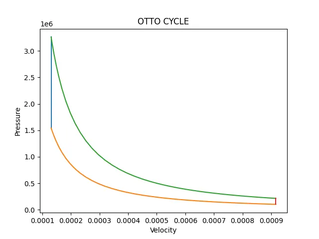
The plot of otto pv has generated by using the above python code.

Conclusion :

I have concluded that ,the otto cycle pv diagram generation and the thermal efficiency has calculated ,by using the python.