Week 2 Air standard Cycle

OBJECTIVES

(1) Write a python code to create a PV diagram.

(2) Take output of python to calculate thermal efficiency of the engine.

PROBLEM STATEMENT

A petrol engine works on Otto cycle which consists of four stages which can be plotted in a pressure-volume (PV) diagram. This PV diagram can be used to gain many insightful inforamation about the whole process of working of petrol engine like thermal efficiency, compression ratio, swept volume, etc.

SOLUTION PROCEDURE

(I) Theory

Otto cycle can be used to convert chemical energy of petrol into mechnical energy through its combustion in an internal cobustion engine of mainly either two stroke or four stroke engine in automobile industries to run cars, motorcycles, etc. Figure 01 shows the internal motion of different parts of (a) two stroke engine and (b) four stroke engine. Here, translatory motion of piston is converted into rotary motion to run flywheel and ultimtely the wheels of the automobile. Inlet and outlet valves are used for suction and exhaust of working fluid (petrol and air) and exhaust gases respectively. Spark plug is used to ignite this air fuel mixture.

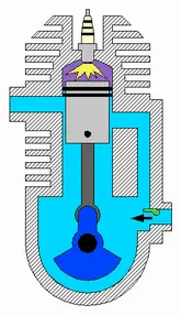
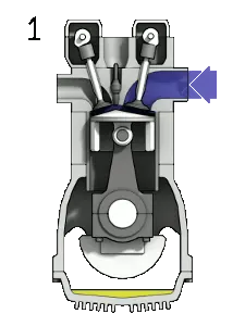
Figure 01. Animation of working of (a) two stroke engine and (b) four stroke engine showing all stages (Source: https://energyeducation.ca/encyclopedia/Otto_cycle ).

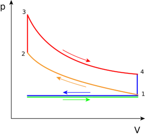
Figure 02: PV diagram of Otto cycle showing different processes (Source: https://energyeducation.ca/encyclopedia/Otto_cycle ).

The entire process of an ideal Otto cycle can be explained by four different stages as shown in FIgure 02.

Suction process (green line): In this stage, piston goes top dead center (TDC) to bottom dead center (BDC) to suck the air-fuel mixture inside the engine cylinder through inlet valve at constant pressure.

Process 1 to 2: Here, piston goes BDC to again TDC to adiabatically compress the air-fuel mixture. During this phase volume decreases and pressure increases with temperature rise of mixture.

Process 2 to 3: Ideally combustion starts at point 2, and it continues till point 3 at constant volume.

Process 3 to 4: It is known a adiabatic expansion stroke. Duringn this process, piston goes from TDC to BDC to give power to engine which is stored into flywheel via crankshaft to run the vehicle.

Process 4 to 1 Exhaust process (blue line): After combustion, the remaining waste gases are passed to atmosphere via exhaust valve at constant volume.

(II) Python code

import math
import matplotlib.pyplot as plt

def engine_kinematics(bore, stroke, con_rod, cr, start_crank, end_crank):
	a = stroke/2
	R = con_rod/a

	v_s = math.pi*(1/4)*pow(bore,2)*stroke
	v_c = v_s/(cr-1)

	sc = math.radians(start_crank) #starting crank angle
	ec = math.radians(end_crank)

	num_values = 100

	dtheta = (ec-sc)/(num_values-1)

	v = []  # empty array to store the value of

	for i in range(0,num_values):
		theta = sc + i*dtheta
		term1 = 0.5*(cr-1)
		term2 = R + 1 - math.cos(theta)
		term3 = pow(R,2) - pow(math.sin(theta),2)
		term3 = pow(term3,0.5)

		v.append((1 + term1*(term2 - term3))*v_c)
	return v

 #volume computation
p1 = 101325
t1 = 450
gamma = 1.4
t3 = 2250
#geoometric parameters

bore = 0.15
stroke = 0.2
con_rod = 0.2
cr = 8 
v_s = math.pi*(1/4)*pow(bore,2)*stroke
v_c = v_s/(cr-1)
v1 = v_c + v_s

 #statepoint 2
v2 = v_c

 #p2v2^gamma = p1v1^gamma
p2 = p1*pow(v1,gamma)/pow(v2,gamma)


#p2v2/t2 = p1v1/t1 | rhs = p1v1/t1 | p2v2/t2 = rhs | t2 = p2v2/rhs

rhs = p1*v1/t1

t2 = p2*v2/rhs
v_compression = engine_kinematics(bore,stroke,con_rod,cr,180,0)

costant = p1*pow(v1,gamma)
p_compression = []
for v in v_compression:
	p_compression.append(costant/pow(v,gamma))

#state point 3

v3 = v2

#p3v3/t3 = p2v2/t2 | rhs = p2v2/t2 | p3 = rhs*t3/v3

rhs + p2*v2/t2
p3 = rhs*t3/v3

v_expansion = engine_kinematics(bore,stroke,con_rod,cr,0,180)

costant = p3*pow(v3,gamma)
p_expansion = []
for v in v_expansion:
	p_expansion.append(costant/pow(v,gamma))
#state point 4

v4 = v1
#p4vv4^gamma = p3v3^gamma

p4 = p3*pow(v3,gamma)/pow(v4,gamma)

#p4v4/t4 = p3v3/t3M
t4 = p4*v4/rhs

term1 = pow(cr,(gamma-1))
thermal_efficiency = 1 - 1/term1 
print(thermal_efficiency)

#plt.plot([v1,v2,v3,v4,v1],[p1,p2,p3,p4,p1])
plt.plot([v2,v3],[p2,p3])
plt.plot(v_compression,p_compression)
plt.plot(v_expansion,p_expansion)
plt.plot([v4,v1],[p4,p1])
plt.xlabel('Volume (m^3)')
plt.ylabel('Pressure (N/m^2)')
plt.show()
v = engine_kinematics(bore,stroke,con_rod,cr,0,180)

Explanation of python code

(1) Line 1-2: import math and maplot library for mathematical codes and plotting graphs.

(2) LIne 4-28: defie a function engine_kinematics in terms of bore, stroke, con_rod, cr, start_crank and end_crank. Define all the variables with their respective equations like, swept volume, clearance volume, start and end crank angles in radians, etc. At line line 14. Define dtheta at line 15 and, take number of plotting points as 100 for a smooth curve. Empty array with append is used in the followig equation to plot curve;

`V/V_c = 1 + 1/2(cr-1)[R + 1 - costheta - (R^2 - sin^2theta)^(1/2)]`

(3) Line 30-87: values of pressure and volume at different process points 1, 2, 3, and 4 are calculated using state equation for constant volume and adiabatic processes as discussed in the theory part.

(4) Line 89-91: here, thermal efficiency is calculated using following equation

`eta = 1- 1/(cr^(gamma) - 1)`

(5) Line 93-101: PV diagram is plotted with labelling for the defined function in step 01.

RESULTS & DISCUSSION

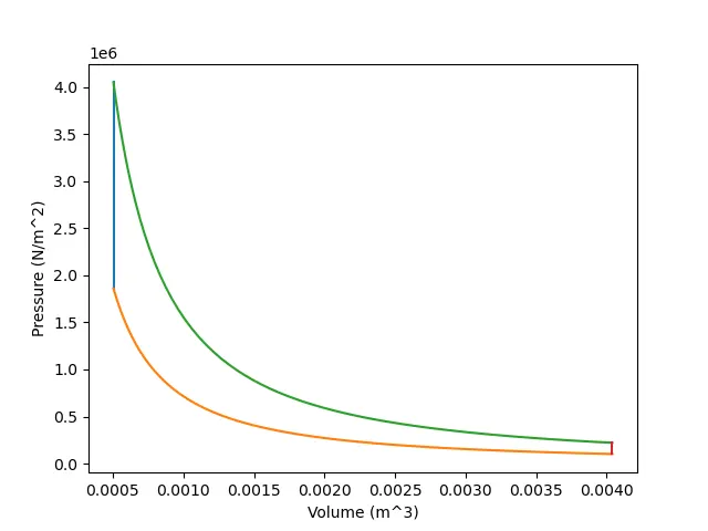
Figure 03. Otto cycle PV diagram

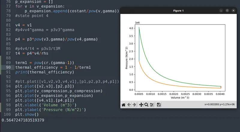
Figure 04. Snapshot of thermal efficiency calculation

Results are plotted in figure 03 and figure 04 for in terms of PV diagram and thermal efficiency. The PV diagram obtained has similar explanation as discussed in the theory part. Thermal efficiency is calculated for ideal Otto cycle using compression ratio.

CONCLUSION

The PV perfectly matches with the theoretical PV diagram discussed in the theory. The thermal efficiency is 56.47%.