Week 3 - Solving second order ODEs

OBJECTIVE

Write a program to solve an Ordinary Differential Equation (ODE) which represents the equation of motion of a simple pendulum with damping.

`(d^2 theta)/dt^2+b/m(d theta)/dt+g/Lsintheta=0` -(1)

PROBLEM STATEMENT

Ordinary differential equations are very important to describe the transient nature of a system. If you can solve these equations then it would pave the path to simulate such a system.

SOLUTION PROCEDURE

1. Theory

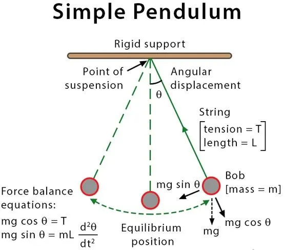
A pendulum is simply a weight which can be in the shape of sphere, it is supended from the pivot and it swings back and forth under the inital displacment and restoring force due to gravity. During oscillation, potential energy and kinetic energy keep interchanging into each other with maximum velocity at mean position and zero velocity at maximum displacement. Galileo Galilei did first scientific observation of it, since then it has been investigated and used for various scientific and commerical applications.

Terminology associated with pendulum:

Length: Distance between the point of pivot to the center of the ball of pendulum.

Time period: It is the time taken by the pendulum to cover one oscillation.

Displacement or angular displacement: It is the disctance or angle covered by ball when displaced from the mean position.

Using above terminologies and Newton's second law, the equation of motion for the pendulum can be written as mentioned in the Aim of this challenge.

2. Steps to be followed

Step 01: Break higher-order ODE into smaller-order ODE. In the present case, it is second-order ODE, so first, break it into a single order.

`theta = theta_1`

`(d theta)/dt=(d theta_1)/dt= theta_2`

So equation (1) can be written as

`(d theta_2)/dt+b/mtheta_2+g/Lsintheta_1=0`

Step 02: Now we have two ODE of single order which are easy to solve

`(d theta_1)/dt= theta_2` &

`(d theta_2)/dt=-b/mtheta_2-g/Lsintheta_1`

Step 03: Write above two equations into a matrix form

`d/dt[[theta_1],[theta_2]]=[[theta_2],[-b/mtheta_2-g/Lsintheta_1]]`

Step 04: Now these equations can be solved.

Step 05: Write code in python to plot a graph for angular displacement, angular velocity and time.

Step 06: Then extend the same code to build an animation by saving pictures for evenly distributed pictures between time steps 0-20 seconds with the help of ImageJ.

3. Python Code:

import numpy as np
from scipy.integrate import odeint
import matplotlib.pyplot as plt
import math

#a function that returns dtheta/dt
def model(theta,t,b,g,L,m):

	theta1 = theta[0]
	theta2 = theta[1]
	dtheta1_dt = theta2
	dtheta2_dt = -(b/m)*theta2 - (g/L)*math.sin(theta1)
	dtheta_dt = [dtheta1_dt, dtheta2_dt]
	return dtheta_dt


b = 0.05
g = 9.81
L = 1
m = 1

#initial conndition
theta_0 = [0,3]

#time points
t = np.linspace(0,20,200)

#solve ODE
theta = odeint(model,theta_0,t,args = (b,g,L,m))

#plot results
plt.plot(t,theta[:,0],'b-',label=r'$\frac{d\theta_1}{dt}=\theta_2$')
plt.plot(t,theta[:,1],'r--',label=r'$\frac{d\theta_2}{dt}=-\frac{b}{m}\theta_2-\frac{g}{L}sin\theta_1$')
plt.title('Angular displacement & Angular velocity vs Time graph')
plt.ylabel('Plot')
plt.xlabel('time')
plt.legend(loc='best')
plt.savefig('Output.png')
plt.show()

###Draw animation
t=1
x0 = 0
y0 = 0

for i in theta[:,0]:
	x1 = (1*math.sin(i))
	y1 = (-1*math.cos(i))

	filename = 'test%05d.png' % ct
	ct = ct +1

	plt.figure()
	plt.plot([-1,1],[0,0],"black",linewidth = 10)
	plt.plot([x0,x1],[y0,y1],"red")
	plt.plot(x1,y1,'o',markersize = 20)
	plt.xlim([-1.5,1.5])
	plt.ylim([-1.5,1.0])
	plt.savefig(filename)

4. Explanation of the python code

Now we need to write a code/program in python that includes all these input varibales and can solve these two ODEs. Here solving ODEs means intergration to get the values of variables involved.

The code in python is written in the following stages:

Step01: Import numpy library/model and odeint library from scipy.integrate model for time step array and solvinf ODEs respectively. Matplotlib.pyplot and math libraries are imported to plot graph and do mathematical calculations respectively.

Step 02: Define function named as model which includes equation of motion and its first order simplified version.

Step 03: Define all the variables, take angular velocity 0-3 rad/sec. Use linspace to equally divide the time interva of 20 seconds into 200 equal parts.

Step 04: Plot the graph with all legends, title, labels, etc.

Step 05: At the end collect the all 200 pictures captured for all 200 time steps and draw animation using ImageJ tool in Linux Ubuntu.

RESULTS & DISCUSSIONS

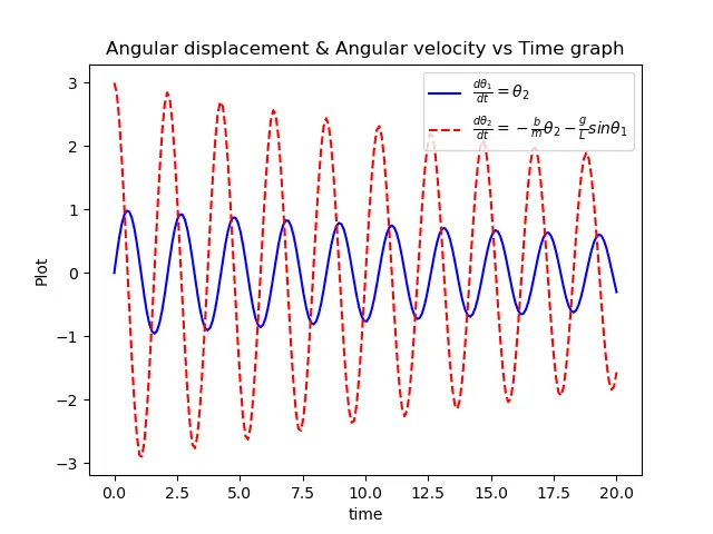
YouTube video link for pendulum oscillation:

https://youtu.be/NWvrFDy2sBQ

CONCLUSION

Oscillation the pendulum strongly depends on the damping coefficients. Larger the damping more rapidly the oscillation will die out. Similarly, length and mass also play significant role. Python code can be written to capture this oscillation.