Week 5 - Curve fitting
1. What does popt and pcov mean?
Ans. (a) popt- Technically, it is an output argument of curve_fit function which is imported from scipy module, it is used to collect coefficients of taken polynomoal for curve fitting. It is 2D array optimal coefficients of the polynomial whihc have give best curve fitting or for which the sum of squared residuals (discussed in next question no 6) are minimized.
(b) pcov- It is also a similar output argument in 2D array like popt but it is consists of estimated values of coovarinace of coeffcients extracted by popt. It shows uncertainties and correlation between of the polynomial. It is square matrix where diagonal elements give variance of the coefficients while non-diagonal elements give covariance of the coefficients. It can be used to find standard deviation in the given data.
2. What does np.array(temperature) do?
Ans. With the help of numpy module it accesses individual elements of the temperature array. Numpy module can be used to do all kinds of arithamatic operations like addition, substraction, multiplication, division, etc. on each element of an array and between arrays.
3. What does the * in *popt mean?
Ans. Techincally, * means "all". With popt that is- *popt it means it is referring to all the values stored in the array given bby popt. It helps to access all the optimized values.
4. Write code to fit a linear and cubic polynomial for the Cp data. Explain if your results are good or bad.
Ans. Here, a linear or first order polynomial and cubic or third order polynomials will considered and
(1) Linear polynomial for the Cp data curve fitting
#LINEAR CURVE FITTING
import numpy as np
import matplotlib.pyplot as plt
from scipy.optimize import curve_fit

def func(t, a, b): #define function that will be used for curve fitting
	return a*t + b #linear eq

def read_file(): #read temperature and specific heat data from file and define it as another function
	temperature =[] # create empty array for temperature
	cp =[] #empty array for specific heat
	for line in open('data','r'): #open a file with name data in read mode and read line by line
		values = line.split(',') #split the line in data file where comma operatorexist using split function and fill in the bracket give here
		temperature.append(float(values[0])) #first value which is separated by comma is temperature with index zero
		cp.append(float(values[1])) #second is cp with index one, convert it into float then add this data into empty array using append

	return [temperature, cp] #return the values of temp and cp


temperature, cp = read_file() #read temp and cp
popt, pcov = curve_fit(func, temperature, cp) # use func which is a quad eq to set relation btw temperature and cp by curve fit by doing so you will get two ouputs popt (set of coeficients: a,b,c) & pcov (variance & covariance of these parameters)
fit_cp = func(np.array(temperature), *popt) #define new function fit_cp which calculates cp again with temp and popt to test the results

plt.plot(temperature, cp,,linewidth=3) #curve for actual data
plt.plot(temperature, fit_cp,,linewidth=3) #curve for curve fir, both should match
plt.legend(['Actual data','Curve fit by linear eq'])
plt.xlabel('Temperature [K]')
plt.ylabel('Cp [J/kg/K]')

plt.show()
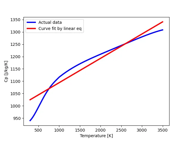
Figure 1. Curve fitting by linear equation
(2) Cubic polynomial for the Cp data curve fitting
#Cubic polynomial for the Cp data curve fitting
import numpy as np
import matplotlib.pyplot as plt
from scipy.optimize import curve_fit

def func(t, a, b, c, d): #define function that will be used for curve fitting
	return a*pow(t,3) + b*pow(t,2) +c*t + d #quadratic eq

def read_file(): #read temperature and specific heat data from file and define it as another function
	temperature =[] # create empty array for temperature
	cp =[] #empty array for specific heat
	for line in open('data','r'): #open a file with name data in read mode and read line by line
		values = line.split(',') #split the line in data file where comma operatorexist using split function and fill in the bracket give here
		temperature.append(float(values[0])) #first value which is separated by comma is temperature with index zero
		cp.append(float(values[1])) #second is cp with index one, convert it into float then add this data into empty array using append

	return [temperature, cp] #return the values of temp and cp


temperature, cp = read_file() #read temp and cp
popt, pcov = curve_fit(func, temperature, cp) # use func which is a quad eq to set relation btw temperature and cp by curve fit by doing so you will get two ouputs popt (set of coeficients: a,b,c) & pcov (variance & covariance of these parameters)
fit_cp = func(np.array(temperature), *popt) #define new function fit_cp which calculates cp again with temp and popt to test the results

plt.plot(temperature, cp,,linewidth=3) #curve for actual data
plt.plot(temperature, fit_cp,,linewidth=3) #curve for curve fir, both should match
plt.legend(['Actual data','Curve fit by cubic eq'])
plt.xlabel('Temperature [K]')
plt.ylabel('Cp [J/kg/K]')

plt.show()
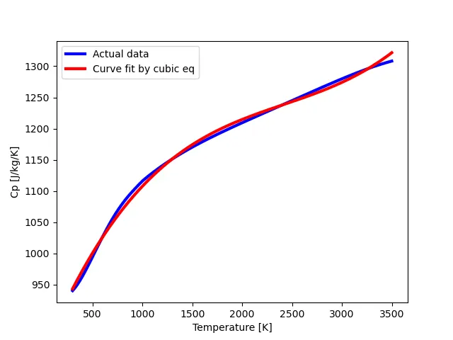
Figure 2. Curve fitting by cubic equation
(c) Explanation of code: The entire code written in python and explained in details in the comments itself, however, it can be summarised in the following points;
1. Import following modules for their corresponding functions: math- mathematical constants, matplotlib- graph plots, numpy- mathematical operations on arrays, optimization function from scipy- to perform curve fitting
2. define funtion - for polynomial equation that will fit the curve as per the trend of data
3. read data from the given file
4. Create empty array for the temperature and specific heat.
5. Open the data in read mode and read it line by line
6. Split the line in data where comma operator exists using split function.
7. Convert both values in float and give index zero to temperature and index one to specific heat and return their values.
8. use popt for optimal cofficient values, pcov for covariance of these coefficients as an output arguments.
9. Define a new function that will calculates cp again with temperature and popt to test the results
10. Plot the grpahs with proper labelling.
(d) Explanation of graphs
From Figure 1 and Figure we can see that cubic equation give more closeness with the data and curve is more near or almost close to the data points with minimum errors in case of cubic equation.
(e) Quatitative analysis of curve fitting: wether curve fitting was good or bad
import math
import matplotlib.pyplot as plt
import numpy as np
from scipy.optimize import curve_fit


def read_file():
	temperature = []
	cp = []
	for line in open('data', 'r'):
		values = line.split(',')
		temperature.append(float(values[0]))
		cp.append(float(values[1]))

	return[temperature, cp]

temperature, cp = read_file()

temperature, cp = read_file()

def linear(T, a, b):
	return(a*T + b)


#linear equation curve fitting
popt1, pcov1 = curve_fit(linear, temperature, cp)
linear_fit_cp = linear(np.array(temperature), *popt1)

#Maximum Percentage Error
error1 = (np.array(np.array(cp) - np.array(linear_fit_cp)))*100/(np.array(cp))
max_error1 = max(error1)
print('Maximum Percentage Error with linear eq =', max_error1)
print('n')


def cubic(T, a, b, c, d):
	return(a*pow(T, 3) + b*pow(T, 2) + c*T + d)


#cubic equation curve fitting
popt2, pcov2 = curve_fit(cubic, temperature, cp)
cubic_fit_cp = cubic(np.array(temperature), *popt2)

#Maximum Percentage Error
error2 = (np.array(np.array(cp) - np.array(cubic_fit_cp)))*100/(np.array(cp))
max_error2 = max(error2)
print('Maximum Percentage Error with cubic eq =', max_error2)
Explanation of code & results
All code lines are similar to previously explained codes for curve fitting except a maximum percentage error is calculated for both linear and cubic curve fitting. Here, it is calculated by taking maximum value from the array of error 1 and 2, which itself is calculated from arrays cp and linear_fit_cp.
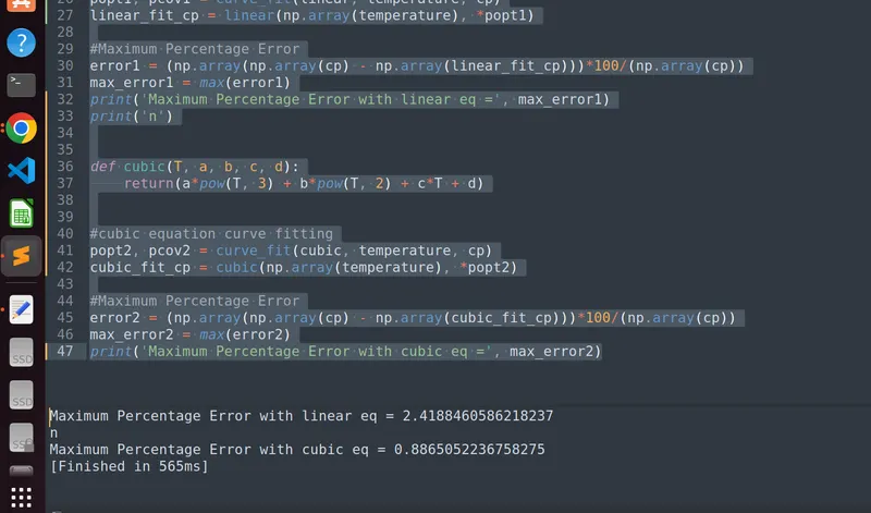
Figure 3 Maximum percentage errrors for linear and cubic curve fitting
Above figure shows that linear curve fitting has error of 2.4% while cubic curve fitting has error of only 0.886%, which shows that cubic eq is better choice than linear equation.
5. What needs to be done in order to make the curve fit perfect?
Ans. There are two ways bywhich a perfect curve fir can be obatined:
(1) Degree of polynomial: A higher degree of polynomial always gives better curve fit than lower degree of polynomial equation. It can be seen in Figure 1 & 2 also, where a cubic equation curve fit is more closer to the acutal data curve than linear polynomial equation.
(2) Split-wise method: In thismethod the whole data is splitted into small parts and then curve fitting is applied to these parts individually. Here, for the same polynomial equation the split-wise method will give perfect fit as every point in curve fit consides with the original data.
import math
import matplotlib.pyplot as plt
import numpy as np
from scipy.optimize import curve_fit


def read_file():
	temperature = []
	cp = []
	for line in open('data', 'r'):
		values = line.split(',')
		temperature.append(float(values[0]))
		cp.append(float(values[1]))

	return[temperature, cp]

temperature, cp = read_file()


#Range[1 - 400]
temperature1 = temperature[0:400]
cp1 = cp[0:400]

#Range[401 - 800]
temperature2 = temperature[400:800]
cp2 = cp[400:800]

#Range[801 - 1200]
temperature3 = temperature[800:1200]
cp3 = cp[800:1200]

#Range[1201 - 1600]
temperature4 = temperature[1200:1600]
cp4 = cp[1200:1600]

#Range[1601 - 2000]
temperature5 = temperature[1600:2000]
cp5 = cp[1600:2000]

#Range[2001 - 2400]
temperature6 = temperature[2000:2400]
cp6 = cp[2000:2400]

#Range[2401 - 2800]
temperature7 = temperature[2400:2800]
cp7 = cp[2400:2800]

#Range[2801 - 3200]
temperature8 = temperature[2800:3200]
cp8 = cp[2800:3200]


def cubic(T, a, b, c, d):
	return(a*pow(T, 3) + b*pow(T, 2) + c*T + d)


#Range[1 - 400]
popt1, pcov1 = curve_fit(cubic, temperature1, cp1)
splitwise_cubic_fit_cp1 = cubic(np.array(temperature1), *popt1)

#Range[401 - 800]
popt2, pcov2 = curve_fit(cubic, temperature2, cp2)
splitwise_cubic_fit_cp2 = cubic(np.array(temperature2), *popt2)

#Range[801 - 1200]
popt3, pcov3 = curve_fit(cubic, temperature3, cp3)
splitwise_cubic_fit_cp3 = cubic(np.array(temperature3), *popt3)

#Range[1201 - 1600]
popt4, pcov4 = curve_fit(cubic, temperature4, cp4)
splitwise_cubic_fit_cp4 = cubic(np.array(temperature4), *popt4)

#Range[1601 - 2000]
popt5, pcov5 = curve_fit(cubic, temperature5, cp5)
splitwise_cubic_fit_cp5 = cubic(np.array(temperature5), *popt5)
#Range[2001 - 2400]
popt6, pcov6 = curve_fit(cubic, temperature6, cp6)
splitwise_cubic_fit_cp6 = cubic(np.array(temperature6), *popt6)

#Range[2401 - 2800]
popt7, pcov7 = curve_fit(cubic, temperature7, cp7)
splitwise_cubic_fit_cp7 = cubic(np.array(temperature7), *popt7)

#Range[2801 - 3200]
popt8, pcov8 = curve_fit(cubic, temperature8, cp8)
splitwise_cubic_fit_cp8 = cubic(np.array(temperature8), *popt8)


#Creation of splitwise_cubic_fit_cp array
splitwise_cubic_fit_cp = np.concatenate((splitwise_cubic_fit_cp1, splitwise_cubic_fit_cp2, splitwise_cubic_fit_cp3, splitwise_cubic_fit_cp4, splitwise_cubic_fit_cp5, splitwise_cubic_fit_cp6, splitwise_cubic_fit_cp7, splitwise_cubic_fit_cp8))

#Maximum Percentage Error
error = (np.array(np.array(cp) - np.array(splitwise_cubic_fit_cp)))*100/(np.array(cp))
max_error = max(error)


#Comparison with original data
plt.figure()

plt.plot(temperature, cp, color = 'r', linewidth = 2, label = 'Original Data')
plt.plot(temperature, splitwise_cubic_fit_cp, color = 'b', linewidth = 2, label = 'Curve Fit')

plt.title('Split-wise method', color = 'k', fontsize = 15, fontweight = 'bold')

plt.xlabel('Temperature [K]', fontsize = 12)
plt.ylabel('Specific Heat [kJ/kg-K]', fontsize = 12)

plt.legend(loc = 'lower right')


plt.text(200, 1300, 'Maximum Percentage Error =' +  str(max_error) + '%', color = 'r', fontsize = 7, fontweight = 'bold')

plt.show()
Explanation of split-wise method code & results
1. Upto code line 20, everything is similar, importing modules, defining function, reading file, and preparing data for curve fitting.
2. Now again read file and this time divide the temperature and cp arrays fro 8 different ranges in code line 30 to 59.
3. define a similar cubic function
4. Do curve fitting for each range using splitwise method
5. Create splitwise curve fit array.
6. Claculate maximum percentage errror.
7. Compare original data by creating plot
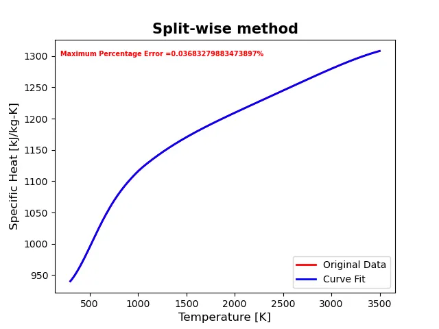
Figure 4. Split-wise method for further improvement over cubic curve fitting
Clearly, Figure 4 shows that even with cubic equation curve fitting, the error has further reduced to 0.036% and curve looks perfectly overlapping with the original data.
6. Show empirically as to how well your curve has been fit.
Ans. In curve fitting we draw a curve that fits closest possible pattern of the given data. It helps to develop a trend or relationship between dependent and independent variables.
There are four possible ways to empirically evaluate how well the curve fit with the given data:
(a) Sum of Squares Residual Errors (SSE), Sum of Square Total (SST), and Sum of Square Regression (SSR)
(b) R-square
(c) Adjusted R-square
(d) Root Mean Squared Error (RMSE)
(a) SSE, SST and SSR
SSE is the sum of squared difference between predicted values and actual values of the given data points. SST is the sum of squared difference between actual values and mean of actual values. SSR is the sum of squared difference between the predicted values and mean of actual values.
Error`= |y(i)-f(x(i))|`
While, SSE`=sum"Error"(i)^2`
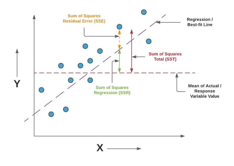
Figure 5. Sum of Squares Residual Errors for curve fitting evaluation
Now, lets say we pupose a nth order polynominal equation that will fit this curve as;
`f(x)=c_1+c_2x+c_3x^2+...+c_nx^(n-1)`
Differentiate SSE with each coefficient of `f(x)` and equate it to zero to get minimum value and corresponding coefficient.
SImilarly other squared errors SST and SSR can be calculated.
From figure 1 it can be said that;
SST = SSR + SSE
(b) R-square
It is the ratio of the SSR to SST, higher the value of R-square better is the curve and vice-versa. Its value ranges from 0 to 1.
`R^2=1-"SSR"/"SST"`
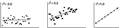
Figure 6. R-square method fot evaluation of curve fitting
(c) Adjusted R-square
R-square value is sometime misleading, for example in case of larger number of parameters R-square value can come out near to 1 as compared to the problem or function with less number of parameters. In that case adjusted R-square is the right way to judge the fitness of curve which is given as;
`"Adjusted" R^2=1-(("SSR"/(n-K))/("SST"/(n-1)))`
Here, n is the number of data points and K is the number of parameters fit.
In case of higher number of parameters, adjusted R-square will be always lower than normal R-square value.
(d) Root Mean Squared Error (RMSE)
`"RMSE"=sqrt("SSE"/n)`
where, n is number of independent variables.
HIgher the value of RMSE better is the curve fitting.
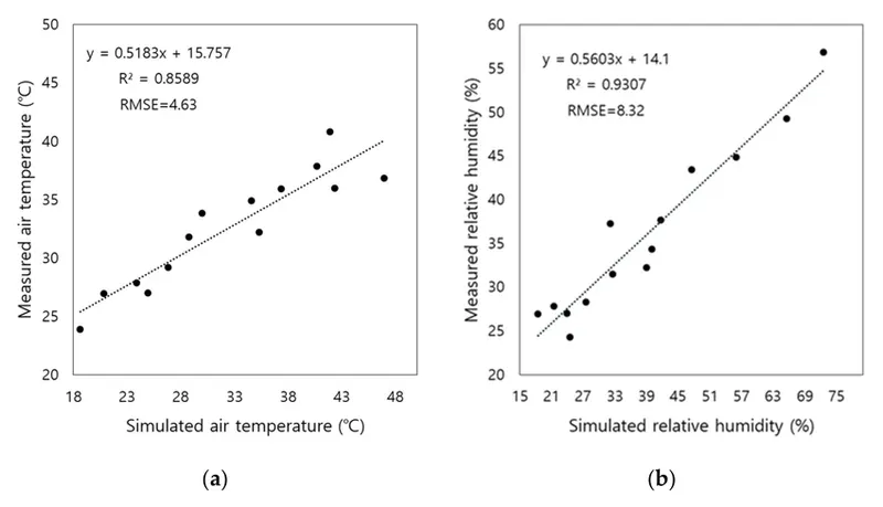
Figure 7 RMSE plot for measured air temperature and measured relative humidity versus simulated air temperature and relative humidity respectively.
Python code for empirical analyis
#Program for empirical analysis
import math
import matplotlib.pyplot as plt
import numpy as np
from scipy.optimize import curve_fit

def read_file():
	temperature = []
	cp = []

	for line in open('data', 'r'):
		values = line.split(',')
		temperature.append(float(values[0]))
		cp.append(float(values[1]))

	return[temperature, cp]

temperature, cp = read_file()

n = len(temperature)
k = 0

def linear(T, a, b):
	return(a*T + b)

popt1, pcov1 = curve_fit(linear, temperature, cp)
linear_fit_cp = linear(np.array(temperature), *popt1)


#Empirical analysis

print('SSE, R-square, Adjusted R-square and RMSE Values for Polynomial of Degree = 1')
print('n')

#SSE
SSE = np.sum(pow((np.array(np.array(cp) - np.array(linear_fit_cp))), 2))
print('Value of SSE =', SSE)
print('t')

# SSR
SSR = np.sum(pow((np.array(np.array(linear_fit_cp) - np.mean(cp))), 2))

#SST
SST = SSE + SSR

#R-square
R_square = SSR/SST
print('Value of R-square =', R_square)
print('t')

#Adj R-square
Adjusted_R_square = 1 - ((1 - R_square)*(n - 1)/(n - k - 1))
print('Value of Adjusted_R_square =', Adjusted_R_square)
print('t')

#RMSE
RMSE = np.sqrt((np.sum(pow((np.array(np.array(cp) - np.array(linear_fit_cp))), 2)))/n);
print('Value of RMSE =', RMSE)
print('n')
print('t')


#Cubic curve fitting
def cubic(T, a, b, c, d):
	return(a*pow(T, 3) + b*pow(T, 2) + c*T + d)


popt2, pcov2 = curve_fit(cubic, temperature, cp)
cubic_fit_cp = cubic(np.array(temperature), *popt2)


#Empirical analysis
print('SSE, R-square, Adjusted R-square and RMSE Values for Polynomial of Degree = 3')
print('n')

#SSE
SSE = np.sum(pow((np.array(np.array(cp) - np.array(cubic_fit_cp))), 2))
print('Value of SSE =', SSE)
print('t')

#SSR
SSR = np.sum(pow((np.array(np.array(cubic_fit_cp) - np.mean(cp))), 2))

#SST
SST = SSE + SSR

#R-square
R_square = SSR/SST
print('Value of R-square =', R_square)
print('t')

#Adj R-square
Adjusted_R_square = 1 - ((1 - R_square)*(n - 1)/(n - k - 1))
print('Value of Adjusted_R_square =', Adjusted_R_square)
print('t')

#RMSE
RMSE = np.sqrt((np.sum(pow((np.array(np.array(cp) - np.array(cubic_fit_cp))), 2)))/n);
print('Value of RMSE =', RMSE)
print('n')
print('t')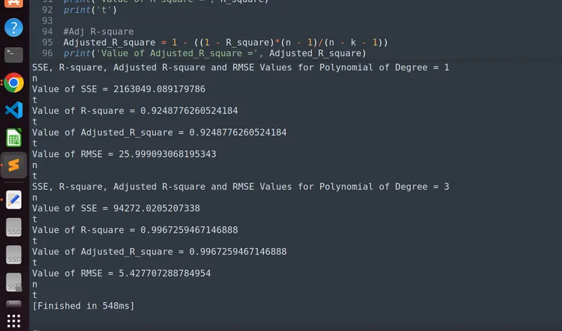
Figure 8. Different types of errors for curve fittinf empirical analysis
Explanation of code & results
Most of the code lines has been already previously discussed, here, new code line are for calculation of SSE, SSR, SST, R-square, Adjusted R-square, and RMSE types of error. For that number independent variables (n) and dashpoints (k) are taken and using sutable formula that have been discussed on the theory part, different types of errors are calculated.
From the Figure 8, we can see that for cubic curve fitting: R-square and adjusted R-square is close to 1 as compared to the linear curve fitting, which proves that increasing order of equation taken for curve fitting improves the results.