Week 2 Air standard Cycle

AIM: To run a program in PYTHON that can solve an otto cycle and make plots for it. Plotting the PV diagram and finding the thermal efficiency of the engine forms the objective of the code.

INTRODUCTION:

Air standard Otto cycle is used for the SI Engines (Spark Ignition Engine). The cycle Contains Mainly four Processes. In the overall cycle, suction and Exhaust are neglected, also power consumption is not considered.
The Ideal Otto cycle consists of the four processes which are as below.

• 1–2 Reversible Adiabatic compression (Or) Isentropic Compression.
• 2–3 Constant Volume Heat Addition.
• 3–4 Reversible Adiabatic Expansion (Or) Isentropic Expansion.
• 4–1 Constant Volume Heat Rejection.
• The PV diagram for a typical otto cycle is as shown in Fig.1

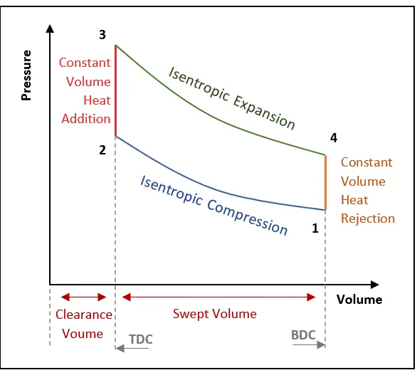
Fig.1 PV diagram of OTTO cycle

Governing Equations:

• Ideal gas equation: `(PV)/T = C` PVT=C
• Isentropic process: `(PV^(GAMMA)) =C`
• Isochoric process: `P/T =C`
• Compression ratio : `(TOTAL VOLUME)/(CLEARANCE VOLUME)`
• Thermal efficiency = 1-1/cr^(gamma-1)
• V/Vc = 1+ 0.5(cr-1)* [ R+1 -cos(theta) — (R² -sin²(theta)^0.5]

CODE:

# OTTO CYCLE SIMULATOR

import math
import matplotlib.pyplot as plt

"""
engine kinematics
"""

def engine(bore,stroke,con_rod,cr,start_crank,end_crank):

#geometric parameters

	a = stroke/2  #crankpin radius
	R = con_rod/a
	 
#volume parameters
	v_s = (math.pi/4)*pow(bore,2)*stroke
	v_c = v_s/(cr-1)

	sc= math.radians(start_crank)
	ec = math.radians(end_crank)    #theta = 0 at top deaad center

	num_values = 50
	dtheta = (ec-sc)/(num_values-1)
	V = []

#***************************************************************************************
#FOR TRACING THE VOLUME CURVE
	for i in range(0,num_values):
		theta = sc + i*dtheta
		term1 = 0.5*(cr-1)
		term2 = R + 1-math.cos(theta)
		term3 =  pow(R,2) - pow(math.sin(theta),2)
		term3 = pow(term3,0.5)

		V.append((1 + term1*(term2-term3))*v_c)

	return V
#***************************************************************************************
#INPUTS
p1 = 101325
t1 = 500

# geometric parameters

bore = 0.1
stroke = 0.1
con_rod = 0.15
cr = 12
gamma = 1.4
t3 = 2300

#***************************************************************************************
#volume computation
#STATE POINT 1 
v_s = (math.pi/4)*pow(bore,2)*stroke
v_c = v_s/(cr-1)

v1 = v_s+v_c

#***************************************************************************************
#state point 2 2-3 is const vol heat additioin
v2 = v_c

#p2v2^gamma = p1v1^gamma
p2 = p1*pow(v1,gamma)/pow(v2,gamma)

#p2v2/t2 = p1v1/t1
rhs = p1*v1/t1
t2 = p2*v2/rhs

V_compression = engine(bore,stroke,con_rod,cr,180,0)
constant = p1*pow(v1,gamma)
P_compression = []

for v in V_compression:
	P_compression.append(constant/pow(v,gamma))

#***************************************************************************************
#state point 3  3-4 is isentropic expansion
v3 = v2

#p3v3/t3 = p2v2/t2
rhs = p2*v2/t2
p3 = rhs*t3/v3


V_expansion = engine(bore,stroke,con_rod,cr,0,180)
constant = p3*pow(v3,gamma)
P_expansion = []

for v in V_expansion:
	P_expansion.append(constant/pow(v,gamma))
#print(p3>p2)

#*************************************************************************************
#state point4 4-1 is cont vol heat rejection
v4 = v1

#p4v4^gamma = p3v3^gamma

p4 = p3*pow(v3,gamma)/pow(v4,gamma)

#p4v4/t4 =rhs  rhs is constant
t4 = p4*v4/rhs

#**************************************************************************************
#plotting pv diagram
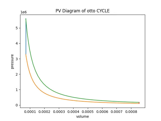
plt.plot([v2,v3], [p2,p3])
plt.plot(V_compression,P_compression)
plt.plot(V_expansion,P_expansion)
plt.plot([v4,v1], [p4,p1])
plt.xlabel('volume')
plt.ylabel('pressure')
plt.title('PV Diagram of otto CYCLE')
plt.savefig('otto CYCLE.png')
plt.show()

#**************************************************************************************
#Thermal efficiency
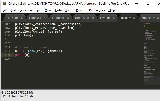
n = 1- (pow(cr,(1-gamma)))
print(n)

CODE EXPLANATION:

• Defining the input variables like gamma, compression ratio, T3.P1.T1 etc.
• Calculating the remaining variables using appropriate relations as per the process involved in moving from one state to another state.
• Now to get the proper curve fitting between the points we make use of the command function in a seperate script and call this function in the main script. The function is given name as engine kinematics and the formula is mentioned here.

V/Vc = 1+ 0.5(cr-1)* [ R+1 -cos(theta) — (R² -sin²(theta)^0.5]

• Corresponding values for P compression, V compression, P expansion and V expansion are calculated for the otto cycle.
• Thermal efficiency calculations are carried out using formula.
• Plot is generated with curve fitting using plot command
• X label, ylabel and title are given to the figure using plt. commands
• Plot is saved as OTTO CYCLE. png using plt.savefile command

RESULTS

CONCLUSION:

• Thermal efficiency is found to be 0.629 or 62.9%
• Python code is compiled without errors and plot is obtained for otto cycle simulation