Week 2 Air standard Cycle

AIM:

1. Your code should create a PV diagram

2. You should output the thermal efficiency of the engine.

OTTO CYCLE PROCESS:

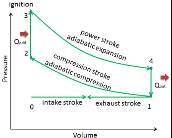
In an ideal Otto cycle, the system executing the cycle undergoes a series of four internally reversible processes: two isentropic (reversible adiabatic) processes alternated with two isochoric processes:

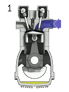
1. Isentropic compression (compression stroke) – The gas (fuel-air mixture) is compressed adiabatically from state 1 to state 2, as the piston moves from bottom dead center to top dead center. The surroundings do work on the gas, increasing its internal energy (temperature) and compressing it. On the other hand the entropy remains unchanged. The changes in volumes and its the ratio (V₁ / V₂) is known as the compression ratio.
2. Isochoric compression (ignition phase) – In this phase (between state 2 and state 3) there is a constant-volume (the piston is at rest ) heat transfer to the air from an external source while the piston is at rest at top dead center. This process is intended to represent the ignition of the fuel–air mixture injected into the chamber and the subsequent rapid burning. The pressure rises and the ratio (P₃ / P₂) is known as the “explosion ratio”.
3. Isentropic expansion (power stroke) – The gas expands adiabatically from state 3 to state 4, as the piston moves from top dead center to bottom dead center. The gas does work on the surroundings (piston) and loses an amount of internal energy equal to the work that leaves the system. Again the entropy remains unchanged. The volume ratio (V₄ / V₃) is known as the isentropic expansion ration, but for Otto cycle, it is equal to the compression ratio.
4. Isochoric decompression (exhaust stroke) – In this phase the cycle completes by a constant-volume process in which heat is rejected from the air while the piston is at bottom dead center. The working gas pressure drops instantaneously from point 4 to point 1. The exhaust valve opens at point 4. The exhaust stroke is directly after this decompression. As the piston moves from bottom dead center (point 1) to top dead center (point 0) with the exhaust valve opened, the gaseous mixture is vented to the atmosphere and the process starts anew.

During the Otto cycle, work is done on the gas by the piston between states 1 and 2 (isentropic compression). Work is done by the gas on the piston between stages 3 and 4 (isentropic expansion). The difference between the work done by the gas and the work done on the gas is the net work produced by the cycle and it corresponds to the area enclosed by the cycle curve. The work produced by the cycle times the rate of the cycle (cycles per second) is equal to the power produced by the Otto engine.

PYTHON CODE:

The detailed explanation about each code is given side by side using # command

import math
import matplotlib.pyplot as plt

#bore and stroke values of a F1 car

b = 0.085   #b - bore, s- stroke
s = 0.065   #b - bore, s- stroke
g = 1.4 #heat capacity ratio
con_rod = 0.05  #conecting rod length
a = s/2
R = con_rod/a
cr = 5  #compression ratio


vs = (3.14/4)*pow(b,2)*s  	 #vs - swept volume
vc = vs/(cr-1)            	 #vc - volume after compression 

# STATE 1 TO 2 - ISENTROPIC COMPRESSION
# STATE 2 TO 3 - ISOCHORIC HEAT ADDITION
# STATE 3 TO 4 - ISENTROPIC EXPANSION
# STATE 4 TO 1 - ISOCHORIC HEAT REJECTION

#STATE 1

p1 = 101325					#atmospheric pressure
t1 = 298					#atmospheric temperature

v1 = vc+vs   				#vc-clearance volume, vs-swept volume


#STATE 2

#p1v1^g = p2v2^g

X = p1*pow(v1,g)			#deriving constant for p1v1^g
v2 = vc 					#volume after compresssion
p2 = X/pow(v2,g)			# pressure at state 2

#p1v1/t1 = p2v2/t2

lhs = p1*v1/t1
t2 = p2*v2/lhs				# temperature at state 2

#v_compression and p_compression

V_compression = []			# V_compression is assigned an empty array so that the volume trace can be found using the volume trace formula and append later
P_compression = []			# P_compression is assigned an empty array so that the V_compression can be used to find P_compression trace and append later

N = 100						# number of variables to smoothen the curve

for i in range(0,N):
	theta1 = (math.pi) - ((math.pi*i)/(N-1))	#logic to get the values from crank angle 180 deg to 0 deg (BDC to TDC)

	#VOLUME TRACE FORMULAE

	term1 = 0.5*(cr-1)
	term2 = R+1-math.cos(theta1)
	term3 = pow(R,2)-pow(math.sin(theta1),2)
	term3 = pow(term3,0.5)

	v_c = (1+term1*(term2-term3))*vc
	V_compression.append(v_c)		#The volume during compression is append to the empty array V_compression

	p_c = X/pow(v_c,g)
	P_compression.append(p_c)		#The pressure during compression is append to the empty array P_compression


#STATE 3

v3 = v2			# VOLUME AT STATE 3
t3 = 2500		# MAXIMUM TEMPERATURE OF THE OTTO CYCLE AT STATE 3

p3=(lhs*t3)/v3	



#STATE 4
#p3v3^g = p4v4^g

v4=v1				#ISOBARIC HEAT REJECTION V4 = V1
TT = p3*pow(v3,g)	#TT is a constant to solve for LHS
p4=TT/pow(v4,g)		# Pressure at state 4

#p3v3/t3 = p4v4/t4

Y = (p3*v3/t3)		# constant to find T4
t4 = p4*v4/Y 		# TEMPERATURE AT STATE4 

#v_expansion and p_expansion

V_expansion = []    # V_expansion is assigned an empty array so that the volume trace can be found using the volume trace formula and append later
P_expansion = []	# P_expansion is assigned an empty array so that the V_expansion can be used to find P_expansion trace and append later

for j in range(0,100):				#logic to get the values from crank angle 0 deg to 180 deg (TDC to BDC)
	theta2 = (math.pi*j)/(N-1)

	
	term1 = 0.5*(cr-1)
	term2 = R+1-math.cos(theta2)
	term3 = pow(R,2)-pow(math.sin(theta2),2)
	term3 = pow(term3,0.5)

	

	v_e = (1+term1*(term2-term3))*vc
	V_expansion.append(v_e)				#The volume during expansion is append to the empty array V_compression

	p_e = TT/pow(v_e,g)
	P_expansion.append(p_e)				#The pressure during expansion is append to the empty array P_compression

#THERMAL EFFICIENCY OF AN OTTO CYCLE FORMULA


EFF = 1 - (1/pow(cr,g-1))

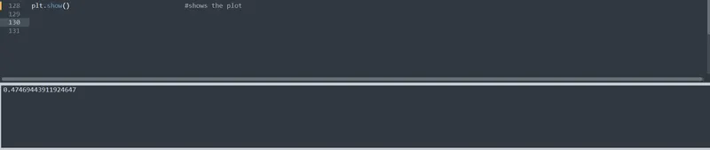
print(EFF)							# PRINTS THE THERMAL EFFICIENCY OF THE OTTO CYCLE

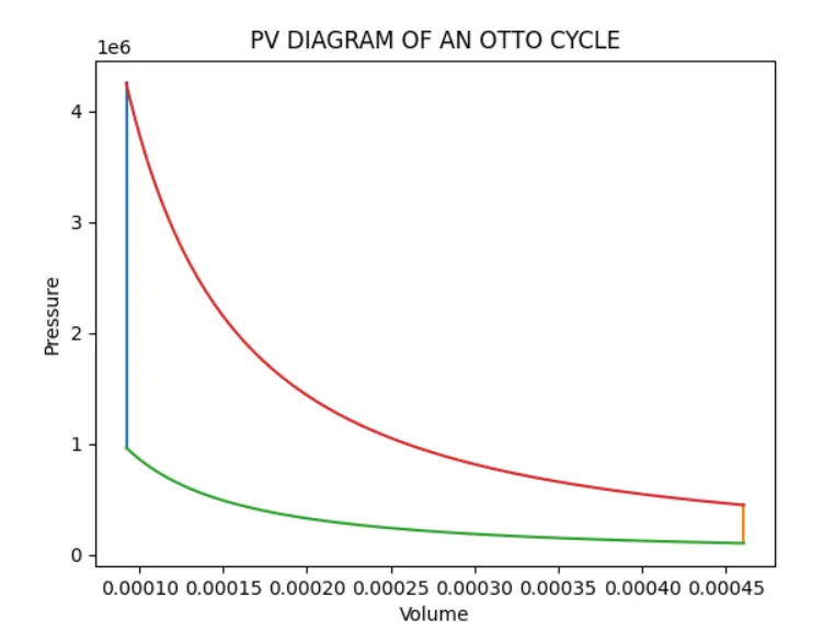
plt.plot([v2,v3],[p2,p3])				# plots the straight line between state 2 and state 3
plt.plot([v4,v1],[p4,p1])				# plots the straight line between state 4 and state 1
plt.plot(V_compression,P_compression)	# plots the curved line between state 1 and state 2
plt.plot(V_expansion,P_expansion)		# plots the curved line between state 3 and state 4

plt.xlabel('Volume')
plt.ylabel('Pressure')
plt.title('PV DIAGRAM OF AN OTTO CYCLE')


plt.show()								#shows the plot

RESULTS :

PV DIAGRAM:

THERMAL EFFICIENCY: